Generalized Hyperbolic Distribution
dist-gh.RdDensity, distribution function, quantile function and random generation for the generalized hyperbolic distribution.
Usage
dgh(x, alpha = 1, beta = 0, delta = 1, mu = 0, lambda = -1/2, log = FALSE)
pgh(q, alpha = 1, beta = 0, delta = 1, mu = 0, lambda = -1/2)
qgh(p, alpha = 1, beta = 0, delta = 1, mu = 0, lambda = -1/2)
rgh(n, alpha = 1, beta = 0, delta = 1, mu = 0, lambda = -1/2)
Arguments
- x, q
a numeric vector of quantiles.
- p
a numeric vector of probabilities.
- n
number of observations.
- alpha
first shape parameter.
- beta
second shape parameter, should in the range
(0, alpha).- delta
scale parameter, must be zero or positive.
- mu
location parameter, by default 0.
- lambda
defines the sublclass, by default \(-1/2\).
- log
a logical flag by default
FALSE. Should labels and a main title drawn to the plot?
Details
dgh gives the density,
pgh gives the distribution function,
qgh gives the quantile function, and
rgh generates random deviates.
The meanings of the parameters correspond to the first
parameterization, pm=1, which is the default parameterization
for this distribution.
In the second parameterization, pm=2, alpha and
beta take the meaning of the shape parameters (usually named)
zeta and rho.
In the third parameterization, pm=3, alpha and
beta take the meaning of the shape parameters (usually named)
xi and chi.
In the fourth parameterization, pm=4, alpha and
beta take the meaning of the shape parameters (usually named)
a.bar and b.bar.
The generator rgh is based on the GH algorithm given
by Scott (2004).
References
Atkinson, A.C. (1982); The simulation of generalized inverse Gaussian and hyperbolic random variables, SIAM J. Sci. Stat. Comput. 3, 502–515.
Barndorff-Nielsen O. (1977); Exponentially decreasing distributions for the logarithm of particle size, Proc. Roy. Soc. Lond., A353, 401–419.
Barndorff-Nielsen O., Blaesild, P. (1983); Hyperbolic distributions. In Encyclopedia of Statistical Sciences, Eds., Johnson N.L., Kotz S. and Read C.B., Vol. 3, pp. 700–707. New York: Wiley.
Raible S. (2000); Levy Processes in Finance: Theory, Numerics and Empirical Facts, PhD Thesis, University of Freiburg, Germany, 161 pages.
Examples
## rgh -
set.seed(1953)
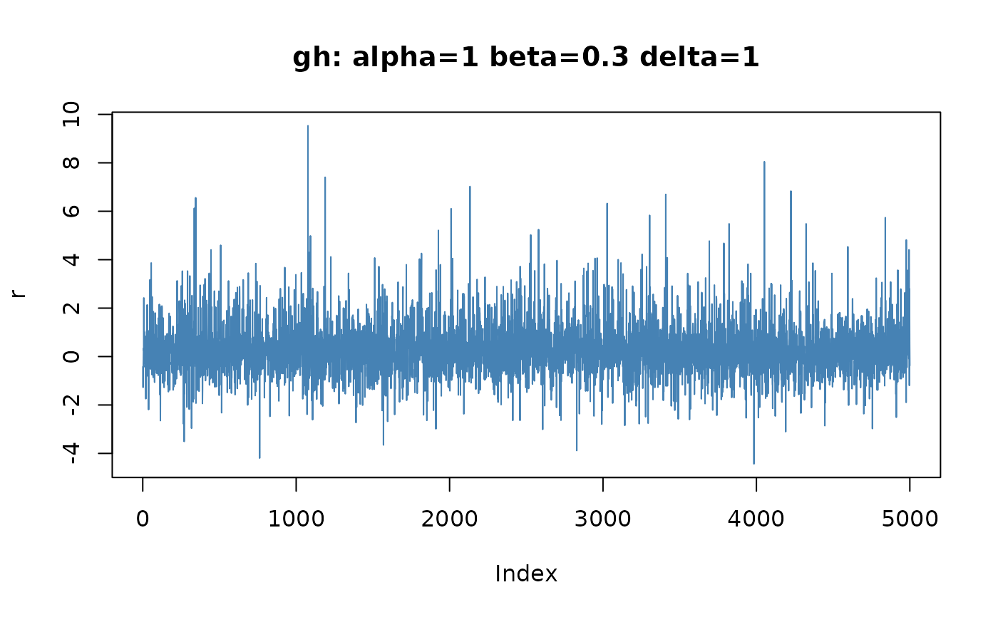
r = rgh(5000, alpha = 1, beta = 0.3, delta = 1)
plot(r, type = "l", col = "steelblue",
main = "gh: alpha=1 beta=0.3 delta=1")
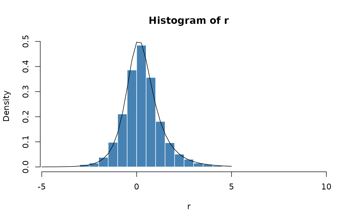
 ## dgh -
# Plot empirical density and compare with true density:
hist(r, n = 25, probability = TRUE, border = "white", col = "steelblue")
x = seq(-5, 5, 0.25)
lines(x, dgh(x, alpha = 1, beta = 0.3, delta = 1))
## dgh -
# Plot empirical density and compare with true density:
hist(r, n = 25, probability = TRUE, border = "white", col = "steelblue")
x = seq(-5, 5, 0.25)
lines(x, dgh(x, alpha = 1, beta = 0.3, delta = 1))
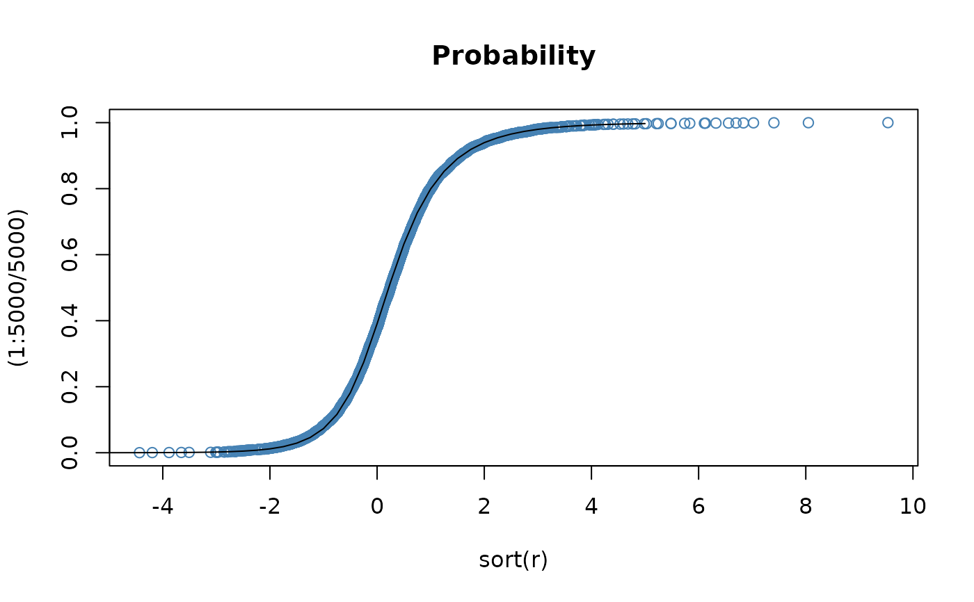
 ## pgh -
# Plot df and compare with true df:
plot(sort(r), (1:5000/5000), main = "Probability", col = "steelblue")
lines(x, pgh(x, alpha = 1, beta = 0.3, delta = 1))
## pgh -
# Plot df and compare with true df:
plot(sort(r), (1:5000/5000), main = "Probability", col = "steelblue")
lines(x, pgh(x, alpha = 1, beta = 0.3, delta = 1))
 ## qgh -
# Compute Quantiles:
qgh(pgh(seq(-5, 5, 1), alpha = 1, beta = 0.3, delta = 1),
alpha = 1, beta = 0.3, delta = 1)
#> [1] -5.000001e+00 -4.000000e+00 -3.000006e+00 -1.999996e+00 -1.000010e+00
#> [6] -8.504243e-06 1.000003e+00 1.999972e+00 3.000000e+00 3.999998e+00
#> [11] 4.999976e+00
## qgh -
# Compute Quantiles:
qgh(pgh(seq(-5, 5, 1), alpha = 1, beta = 0.3, delta = 1),
alpha = 1, beta = 0.3, delta = 1)
#> [1] -5.000001e+00 -4.000000e+00 -3.000006e+00 -1.999996e+00 -1.000010e+00
#> [6] -8.504243e-06 1.000003e+00 1.999972e+00 3.000000e+00 3.999998e+00
#> [11] 4.999976e+00