GH Distribution Fit

Estimates the distrinbutional parameters for a generalized lambda distribution.

Usage

gldFit(x, lambda1 = 0, lambda2 = -1, lambda3 = -1/8, lambda4 = -1/8, 
    method = c("mle", "mps", "gof", "hist", "rob"),
    scale = NA, doplot = TRUE, add = FALSE, span = "auto", trace = TRUE, 
    title = NULL, description = NULL, ...)

Arguments

x

a numeric vector.

lambda1, lambda2, lambda3, lambda4

are numeric values where lambda1 is the location parameter, lambda2 is the location parameter, lambda3 is the first shape parameter, and lambda4 is the second shape parameter.

method

a character string, the estimation approach to fit the distributional parameters, see details.

scale

not used.

doplot

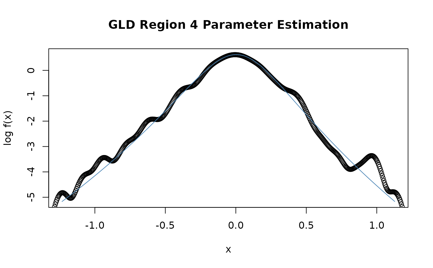
a logical flag. Should a plot be displayed?

add

a logical flag. Should a new fit added to an existing plot?

span

x-coordinates for the plot, by default 100 values automatically selected and ranging between the 0.001, and 0.999 quantiles. Alternatively, you can specify the range by an expression like span=seq(min, max, times = n), where, min and max are the left and rigldt endpoints of the range, and n gives the number of the intermediate points.

trace

a logical flag. Should the parameter estimation process be traced?

title

a character string which allows for a project title.

description

a character string which allows for a brief description.

...

parameters to be parsed.

Details

The function nlminb is used to minimize the objective function. The following approaches have been implemented:

"mle", maximimum log likelihoo estimation.

"mps", maximum product spacing estimation.

"gof", goodness of fit approaches, type="ad" Anderson-Darling, type="cvm" Cramer-vonMise, type="ks" Kolmogorov-Smirnov.

"hist", histogram binning approaches, "fd" Freedman-Diaconis binning, "scott", Scott histogram binning, "sturges", Sturges histogram binning.

"rob", robust moment matching.

Value

an object from class "fDISTFIT". Slot fit is a list, currently with components estimate, minimum and code.

Examples

set.seed(1953)
s <- rgld(n = 1000, lambda1=0, lambda2=-1, lambda3=-1/8, lambda4=-1/8) 

gldFit(s, lambda1=0, lambda2=-1, lambda3=-1/8, lambda4=-1/8, 
       doplot = TRUE, trace = FALSE) 

#> 
#> Title:
#>  GLD Region 4 Parameter Estimation 
#> 
#> Call:
#>  .gldFit.mle(x = x, lambda1 = lambda1, lambda2 = lambda2, lambda3 = lambda3, 
#>     lambda4 = lambda4, scale = scale, doplot = doplot, add = add, 
#>     span = span, trace = trace, title = title, description = description)
#> 
#> Model:
#>  GLD Region 4 Distribution
#> 
#> Estimated Parameter(s):
#>      lambda1      lambda2      lambda3      lambda4 
#>  0.005005736 -0.847892745 -0.110677830 -0.100958859 
#>