Hyperbolic distribution
dist-hyp.RdDensity, distribution function, quantile function and random generation for the hyperbolic distribution.
Usage
dhyp(x, alpha = 1, beta = 0, delta = 1, mu = 0, pm = 1, log = FALSE)
phyp(q, alpha = 1, beta = 0, delta = 1, mu = 0, pm = 1, ...)
qhyp(p, alpha = 1, beta = 0, delta = 1, mu = 0, pm = 1, ...)
rhyp(n, alpha = 1, beta = 0, delta = 1, mu = 0, pm = 1)
Arguments
- x, q
numeric vector of quantiles.
- p
numeric vector of probabilities.
- n
number of observations.
- alpha
-
shape parameter, a positive number.
alphacan also be a vector of length four, containingalpha,beta,deltaandmu(in that order). - beta
-
skewness parameter,
abs(beta)is in the range(0, alpha). - delta
scale parameter, must be zero or positive.
- mu
location parameter, by default 0.
- pm
-
integer number specifying the parameterisation, one of
1,2,3, or4. The default is the first parameterization. - log
-
a logical value, if
TRUE, probabilitiespare given aslog(p). - ...
arguments to be passed to the function
integrate.
Details
dhyp gives the density,
phyp gives the distribution function,
qhyp gives the quantile function, and
rhyp generates random deviates.
The meaning of the parameters given above corresponds to the first
parameterization, pm = 1, which is the default.
In the second parameterization, pm=2, alpha and
beta take the meaning of the shape parameters (usually named)
zeta and rho.
In the third parameterization, pm=3, alpha and
beta take the meaning of the shape parameters (usually named)
xi and chi.
In the fourth parameterization, pm=4, alpha and
beta take the meaning of the shape parameters (usually named)
a.bar and b.bar.
The generator rhyp is based on the HYP algorithm given by
Atkinson (1982).
References
Atkinson, A.C. (1982); The simulation of generalized inverse Gaussian and hyperbolic random variables, SIAM J. Sci. Stat. Comput. 3, 502–515.
Barndorff-Nielsen O. (1977); Exponentially decreasing distributions for the logarithm of particle size, Proc. Roy. Soc. Lond., A353, 401–419.
Barndorff-Nielsen O., Blaesild, P. (1983); Hyperbolic distributions. In Encyclopedia of Statistical Sciences, Eds., Johnson N.L., Kotz S. and Read C.B., Vol. 3, pp. 700–707. New York: Wiley.
Raible S. (2000); Levy Processes in Finance: Theory, Numerics and Empirical Facts, PhD Thesis, University of Freiburg, Germany, 161 pages.
Examples
## hyp -
set.seed(1953)
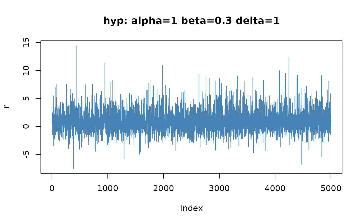
r = rhyp(5000, alpha = 1, beta = 0.3, delta = 1)
plot(r, type = "l", col = "steelblue",
main = "hyp: alpha=1 beta=0.3 delta=1")
 ## hyp -
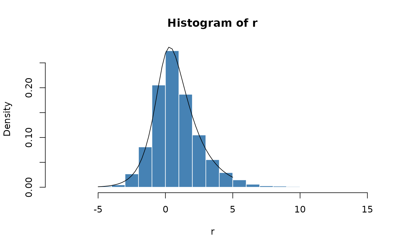
# Plot empirical density and compare with true density:
hist(r, n = 25, probability = TRUE, border = "white", col = "steelblue")
x = seq(-5, 5, 0.25)
lines(x, dhyp(x, alpha = 1, beta = 0.3, delta = 1))
## hyp -
# Plot empirical density and compare with true density:
hist(r, n = 25, probability = TRUE, border = "white", col = "steelblue")
x = seq(-5, 5, 0.25)
lines(x, dhyp(x, alpha = 1, beta = 0.3, delta = 1))
 ## hyp -
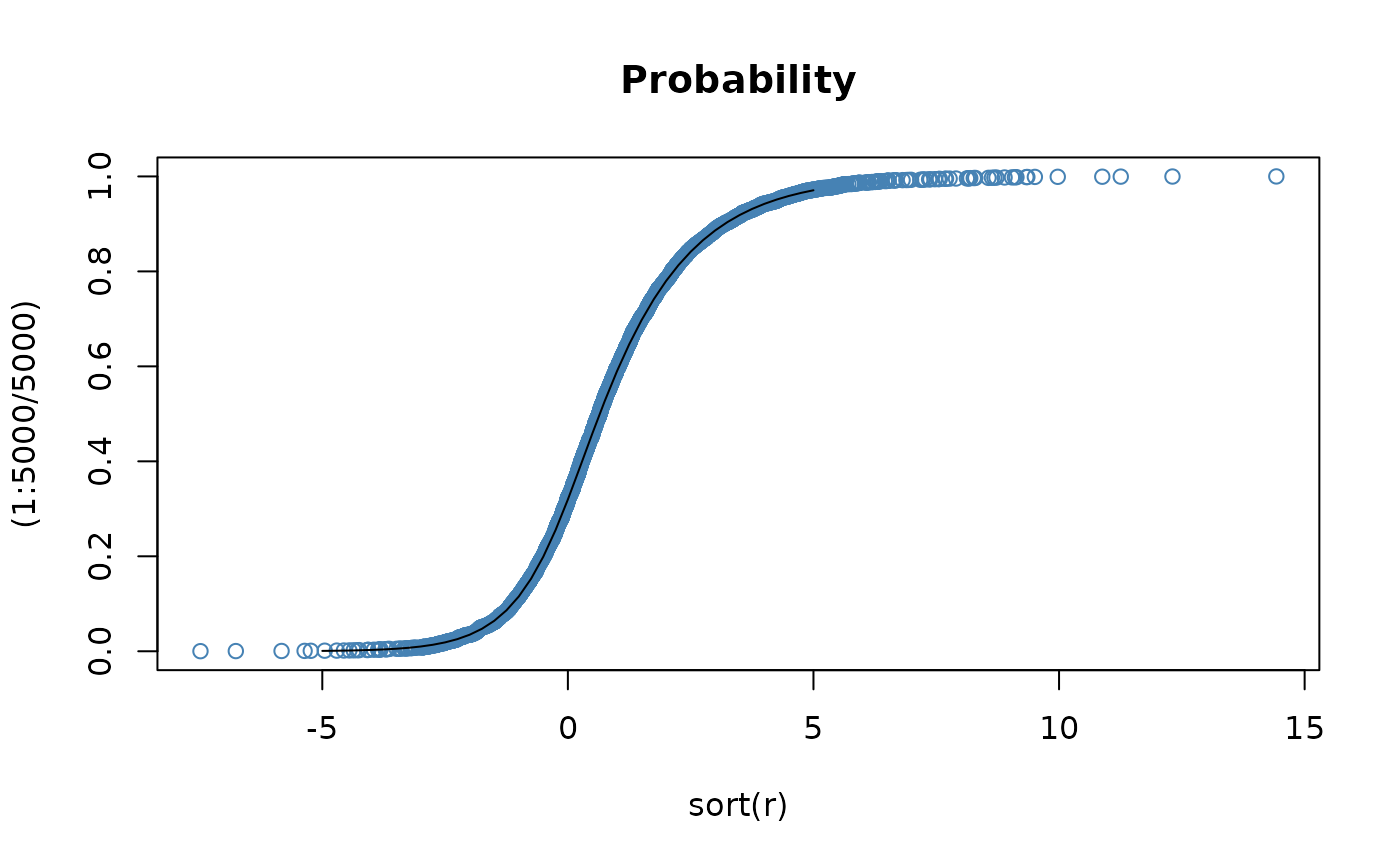
# Plot df and compare with true df:
plot(sort(r), (1:5000/5000), main = "Probability", col = "steelblue")
lines(x, phyp(x, alpha = 1, beta = 0.3, delta = 1))
## hyp -
# Plot df and compare with true df:
plot(sort(r), (1:5000/5000), main = "Probability", col = "steelblue")
lines(x, phyp(x, alpha = 1, beta = 0.3, delta = 1))
 ## hyp -
# Compute Quantiles:
qhyp(phyp(seq(-5, 5, 1), alpha = 1, beta = 0.3, delta = 1),
alpha = 1, beta = 0.3, delta = 1)
#> [1] -5.000017e+00 -3.999997e+00 -3.000000e+00 -2.000023e+00 -1.000003e+00
#> [6] -2.344483e-06 1.000000e+00 2.000000e+00 2.999997e+00 3.999989e+00
#> [11] 5.000002e+00
## hyp -
# Compute Quantiles:
qhyp(phyp(seq(-5, 5, 1), alpha = 1, beta = 0.3, delta = 1),
alpha = 1, beta = 0.3, delta = 1)
#> [1] -5.000017e+00 -3.999997e+00 -3.000000e+00 -2.000023e+00 -1.000003e+00
#> [6] -2.344483e-06 1.000000e+00 2.000000e+00 2.999997e+00 3.999989e+00
#> [11] 5.000002e+00