Standardized generalized hyperbolic Student-t Distribution

Density, distribution function, quantile function and random generation for the standardized generalized hyperbolic Student-t distribution.

Usage

dsght(x, beta = 0.1, delta = 1, mu = 0, nu = 10, log = FALSE)
psght(q, beta = 0.1, delta = 1, mu = 0, nu = 10)
qsght(p, beta = 0.1, delta = 1, mu = 0, nu = 10)
rsght(n, beta = 0.1, delta = 1, mu = 0, nu = 10)

Arguments

x, q

a numeric vector of quantiles.

p

a numeric vector of probabilities.

n

number of observations.

beta

numeric value, beta is the skewness parameter in the range (0, alpha).

delta

numeric value, the scale parameter, must be zero or positive.

mu

numeric value, the location parameter, by default 0.

nu

a numeric value, the number of degrees of freedom. Note, alpha takes the limit of abs(beta), and lambda=-nu/2.

log

a logical, if TRUE, probabilities p are given as log(p).

Details

dsght gives the density, psght gives the distribution function, qsght gives the quantile function, and rsght generates random deviates.

These are the parameters in the first parameterization.

Value

numeric vector

Author

Diethelm Wuertz

Examples

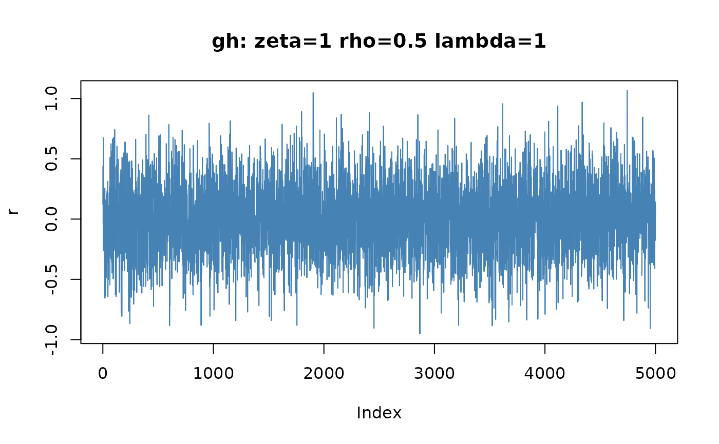
## rsght -
   set.seed(1953)
   r = rsght(5000, beta = 0.1, delta = 1, mu = 0, nu = 10)
   plot(r, type = "l", col = "steelblue",
     main = "gh: zeta=1 rho=0.5 lambda=1")


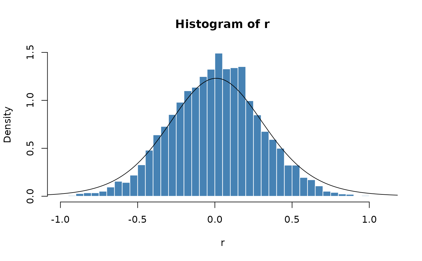
## dsght -
   # Plot empirical density and compare with true density:
   hist(r, n = 50, probability = TRUE, border = "white", col = "steelblue")
   x = seq(-5, 5, length = 501)
   lines(x, dsght(x, beta = 0.1, delta = 1, mu = 0, nu = 10))


## psght -
   # Plot df and compare with true df:
   plot(sort(r), (1:5000/5000), main = "Probability", col = "steelblue")
   lines(x, psght(x, beta = 0.1, delta = 1, mu = 0, nu = 10))


## qsght -
   # Compute Quantiles:
   round(qsght(psght(seq(-5, 5, 1), beta = 0.1, delta = 1, mu = 0, nu =10),
               beta = 0.1, delta = 1, mu = 0, nu = 10), 4)
#>  [1] -5 -4 -3 -2 -1  0  1  2  3  4  5