Standardized Normal Inverse Gaussian Distribution
dist-snig.RdDensity, distribution function, quantile function and random generation for the standardized normal inverse Gaussian distribution.
Usage
dsnig(x, zeta = 1, rho = 0, log = FALSE)
psnig(q, zeta = 1, rho = 0)
qsnig(p, zeta = 1, rho = 0)
rsnig(n, zeta = 1, rho = 0)Details
dsnig gives the density,
psnig gives the distribution function,
qsnig gives the quantile function, and
rsnig generates random deviates.
The random deviates are calculated with the method described by Raible (2000).
Examples
## snig -
set.seed(1953)
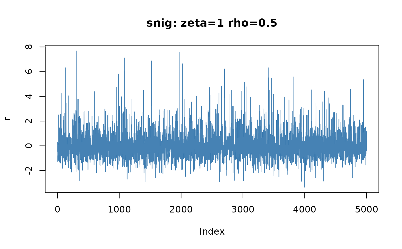
r = rsnig(5000, zeta = 1, rho = 0.5)
plot(r, type = "l", col = "steelblue",
main = "snig: zeta=1 rho=0.5")
 ## snig -
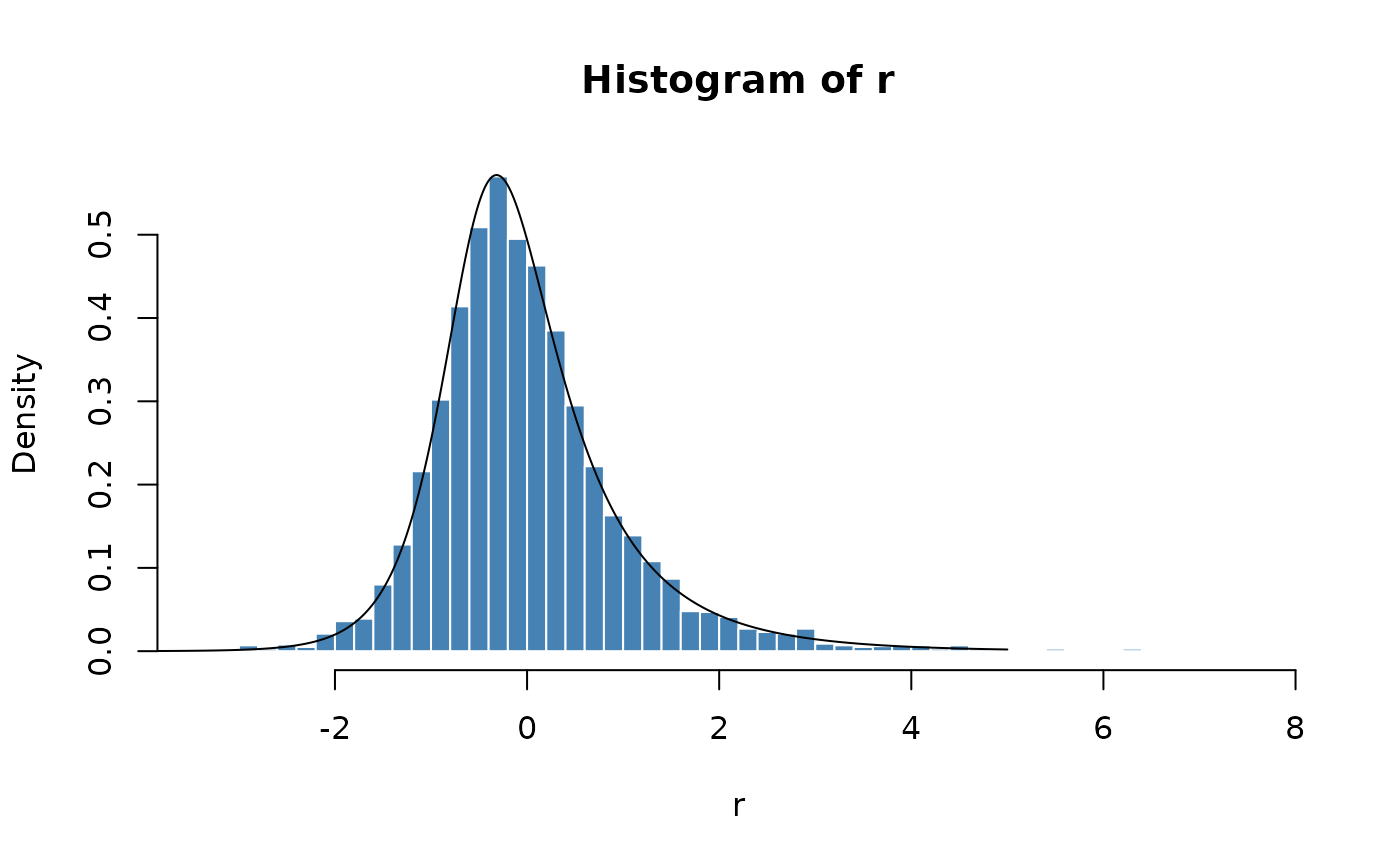
# Plot empirical density and compare with true density:
hist(r, n = 50, probability = TRUE, border = "white", col = "steelblue")
x = seq(-5, 5, length = 501)
lines(x, dsnig(x, zeta = 1, rho = 0.5))
## snig -
# Plot empirical density and compare with true density:
hist(r, n = 50, probability = TRUE, border = "white", col = "steelblue")
x = seq(-5, 5, length = 501)
lines(x, dsnig(x, zeta = 1, rho = 0.5))
 ## snig -
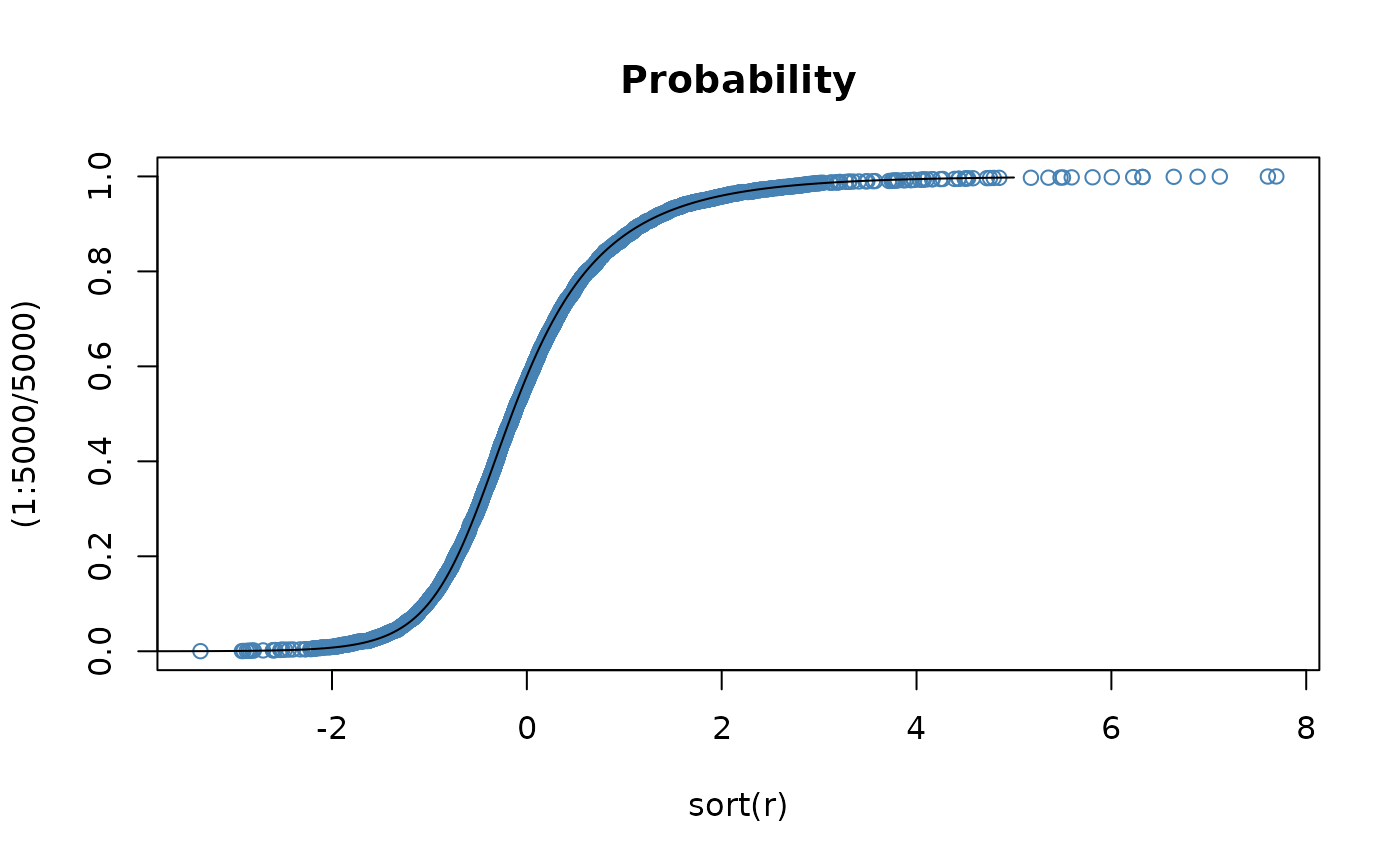
# Plot df and compare with true df:
plot(sort(r), (1:5000/5000), main = "Probability", col = "steelblue")
lines(x, psnig(x, zeta = 1, rho = 0.5))
## snig -
# Plot df and compare with true df:
plot(sort(r), (1:5000/5000), main = "Probability", col = "steelblue")
lines(x, psnig(x, zeta = 1, rho = 0.5))
 ## snig -
# Compute Quantiles:
qsnig(psnig(seq(-5, 5, 1), zeta = 1, rho = 0.5), zeta = 1, rho = 0.5)
#> [1] -5.000000e+00 -3.999999e+00 -2.999983e+00 -2.000011e+00 -1.000000e+00
#> [6] -2.609555e-07 1.000004e+00 2.000016e+00 3.000001e+00 4.000000e+00
#> [11] 5.000029e+00
## snig -
# Compute Quantiles:
qsnig(psnig(seq(-5, 5, 1), zeta = 1, rho = 0.5), zeta = 1, rho = 0.5)
#> [1] -5.000000e+00 -3.999999e+00 -2.999983e+00 -2.000011e+00 -1.000000e+00
#> [6] -2.609555e-07 1.000004e+00 2.000016e+00 3.000001e+00 4.000000e+00
#> [11] 5.000029e+00