Autocorrelation function plots

Returns plots of autocorrelations including the autocorrelation function ACF, the partial ACF, the lagged ACF, and the Taylor effect plot.

The functions to display stylized facts are:

acfPlot	autocorrelation function plot,
pacfPlot	partial autocorrelation function plot,
lacfPlot	lagged autocorrelation function plot,
teffectPlot	Taylor effect plot.

Usage

acfPlot(x, labels = TRUE, ...)
pacfPlot(x, labels = TRUE, ...) 

lacfPlot(x, n = 12, lag.max = 20, type = c("returns", "values"),
    labels = TRUE, ...)

teffectPlot(x, deltas = seq(from = 0.2, to = 3, by = 0.2), lag.max = 10, 
    ymax = NA, standardize = TRUE, labels = TRUE, ...)

Arguments

x

an uni- or multivariate return series of class timeSeries or any other object which can be transformed by the function as.timeSeries() into an object of class timeSeries.

labels

a logical value. Whether or not x- and y-axes should be automatically labeled and a default main title should be added to the plot. By default TRUE.

n

an integer value, the number of lags.

lag.max

maximum lag for which the autocorrelation should be calculated, an integer.

type

a character string which specifies the type of the input series, either "returns" or series "values". In the case of a return series as input, the required value series is computed by cumulating the financial returns: exp(colCumsums(x))

deltas

the exponents, a numeric vector, by default ranging from 0.2 to 3.0 in steps of 0.2.

ymax

maximum y-axis value on plot. If NA, then the value is selected automatically.

standardize

a logical value. Should the vector x be standardized?

...

arguments to be passed.

Details

Autocorrelation Functions:

The functions acfPlot and pacfPlot, plot and estimate autocorrelation and partial autocorrelation function. The functions allow to get a first view on correlations within the time series. The functions are synonym function calls for R's acf and pacf from the the ts package.

Taylor Effect:

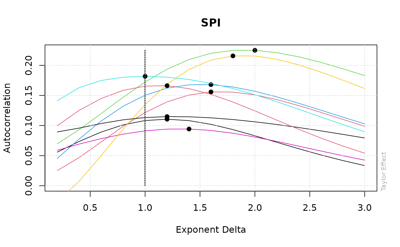
The "Taylor Effect" describes the fact that absolute returns of speculative assets have significant serial correlation over long lags. Even more, autocorrelations of absolute returns are typically greater than those of squared returns. From these observations the Taylor effect states, that that the autocorrelations of absolute returns to the the power of delta, abs(x-mean(x))^delta reach their maximum at delta=1. The function teffect explores this behaviour. A plot is created which shows for each lag (from 1 to max.lag) the autocorrelations as a function of the exponent delta. In the case that the above formulated hypothesis is supported, all the curves should peak at the same value around delta=1.

Value

for acfPlot and pacfplot, an object of class "acf", see acf;

for teffectPlot, a numeric matrix of order deltas by max.lag with the values of the autocorrelations;

for lacfPlot, a list with the following two elements:

Rho

the autocorrelation function,

lagged

the lagged correlations.

References

Taylor S.J. (1986); Modeling Financial Time Series, John Wiley and Sons, Chichester.

Ding Z., Granger C.W.J., Engle R.F. (1993); A long memory property of stock market returns and a new model, Journal of Empirical Finance 1, 83.

Examples

## data
data(LPP2005REC, package = "timeSeries")
SPI <- LPP2005REC[, "SPI"]
plot(SPI, type = "l", col = "steelblue", main = "SP500")
abline(h = 0, col = "grey")


## Taylor Effect:
teffectPlot(SPI)