Scaling law behaviour

Evaluates the scaling exponent of a financial return series and plots the scaling law.

Usage

scalinglawPlot(x, span = ceiling(log(length(x)/252)/log(2)), doplot = TRUE, 
    labels = TRUE, trace = TRUE, ...)

Arguments

x

an uni- or multivariate return series of class "timeSeries" or any other object which can be transformed by the function as.timeSeries() into an object of class "timeSeries".

span

an integer value, determines the plot range. The defaault computes a reasonable number of points for the scaling range, assuming daily data with 252 business days per year.

doplot

a logical value. Should a plot be displayed?

labels

a logical value. Whether or not x- and y-axes should be automatically labeled and a default main title should be added to the plot. By default TRUE.

trace

a logical value. Should the computation be traced?

...

arguments to be passed to plot.

Value

a list with the following components:

Intercept

intercept,

Exponent

the scaling exponent,

InverseExponent

the inverse of the scaling component.

Details

The function scalinglawPlot plots the scaling law of financial time series under aggregation and returns an estimate for the scaling exponent. The scaling behavior is a very striking effect of the foreign exchange market and also other markets expressing a regular structure for the volatility. Considering the average absolute return over individual data periods one finds a scaling power law which relates the mean volatility over given time intervals to the size of these intervals. The power law is in many cases valid over several orders of magnitude in time. Its exponent usually deviates significantly from a Gaussian random walk model which implies 1/2.

References

Taylor S.J. (1986); Modeling Financial Time Series, John Wiley and Sons, Chichester.

Author

Diethelm Wuertz for the Rmetrics R-port

See also

seriesPlot, returnPlot, cumulatedPlot, drawdownPlot

qqnormPlot, qqnigPlot, qqghtPlot, qqgldPlot

histPlot, densityPlot, logDensityPlot

boxPlot, boxPercentilePlot

acfPlot, pacfPlot, teffectPlot, lacfPlot

returnSeriesGUI

Examples

## data
data(LPP2005REC, package = "timeSeries")
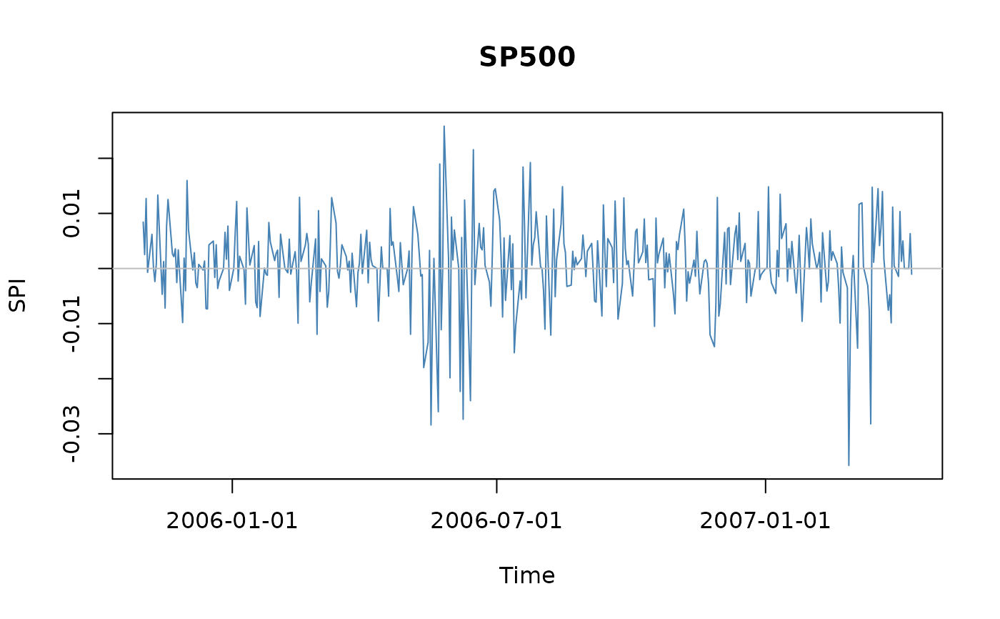
SPI <- LPP2005REC[, "SPI"]
plot(SPI, type = "l", col = "steelblue", main = "SP500")
abline(h = 0, col = "grey")


## Scaling Law Effect
scalinglawPlot(SPI)

#> 
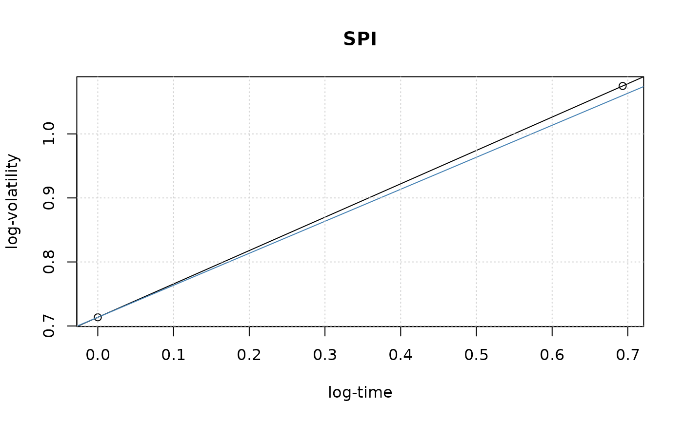#> Scaling Law:          SPI
#>   Plot Intercept      0.7135344
#>   Plot Slope          0.5213102
#>   Plot Inverse Slope  1.918244
#>