Plot 'timeSeries' objects

"timeSeries" methods for plot, lines and points.

Usage

# S4 method for timeSeries
plot(x, y, FinCenter = NULL,
    plot.type = c("multiple", "single"), format = "auto",
    at = pretty(x), widths = 1, heights = 1, xy.labels,
    xy.lines, panel = lines, nc, yax.flip = FALSE,
    mar.multi = c(0, 5.1, 0, if (yax.flip) 5.1 else 2.1),
    oma.multi = c(6, 0, 5, 0), axes = TRUE, ...)

# S4 method for timeSeries
lines(x, FinCenter = NULL, ...)
# S4 method for timeSeries
points(x, FinCenter = NULL, ...)

# S3 method for timeSeries
pretty(x, n=5, min.n=n%/%3, shrink.sml=0.75,
    high.u.bias=1.5, u5.bias=0.5+1.5*high.u.bias, eps.correct=0, ...)

Details

Our original method plot was build along R's plotting function plot.ts with an additional argument to tailor the position marks at user defined position specified by the argument at. We call this style or theme "ts".

With verson R 3.1 we have inroduced two new additional plotting themes called "pretty" and "chick". They are becoming active when we set at = "pretty" or at = "chic".

Plot style or theme "pretty" is an extension of our original plotting method.

Plot style or theme "chic" is an implementation along the contributed packages xts and PerformanceAnalytics from the Chicago finance group members ("chic" is an abbreviation of Chicago.

For both themes, "pretty" and "chic", additional arguments are passed through the ... arguments. These are:

Argument	Default	Description
type	"l"	types pf plot
col	1	colors for lines and points
pch	20	plot symbol
cex	1	character and symbol scales
lty	1	line types
lwd	2	line widths
cex.axes	1	scale of axes
cex.lab	1	scale of labels
cex.pch	1	scale of plot symbols
grid	TRUE	should grid lines plotted?
frame.plot	TRUE	should b box around the plot?
axes	TRUE	should be axes drawn on the plot?
ann	TRUE	should default annotations appear?

Concerning the plot elements, the length of these vectors has to be the same as the number of columns in the time series to be plotted. If their length is only one, then they are repeated.

There is an almost 70 pages vignette added to the package, with dozens of examples of tailored plots. Have a look in it.

Arguments

x, y

objects of class timeSeries.

FinCenter

a character with the the location of the financial center named as "continent/city".

plot.type

for multivariate time series, should the series by plotted separately (with a common time axis) or on a single plot?

format

POSIX label format, e.g. "%Y-%m-%d" or "%F" for ISO-8601 standard date format.

at

a timeDate object setting the plot label positions. If at=pretty(x), the postitions are generated automatized calling the function pretty. Default option at="auto" selects 6 equal spaced time label positions. For the new plot themes set at="pretty" or at="chic". In this case additional arguments can be passed through the ... arguments, see details.

widths, heights

widths and heights for individual graphs, see layout.

xy.labels

logical, indicating if text() labels should be used for an x-y plot, _or_ character, supplying a vector of labels to be used. The default is to label for up to 150 points, and not for more.

xy.lines

logical, indicating if lines should be drawn for an x-y plot. Defaults to the value of xy.labels if that is logical, otherwise to TRUE

panel

a function(x, col, bg, pch, type, ...) which gives the action to be carried out in each panel of the display for plot.type="multiple". The default is lines.

nc

the number of columns to use when type="multiple". Defaults to 1 for up to 4 series, otherwise to 2.

yax.flip

logical indicating if the y-axis (ticks and numbering) should flip from side 2 (left) to 4 (right) from series to series when type="multiple".

mar.multi, oma.multi

the (default) par settings for plot.type="multiple".

axes

logical indicating if x- and y- axes should be drawn.

n

an integer giving the desired number of intervals.

min.n

a nonnegative integer giving the minimal number of intervals.

shrink.sml

a positive numeric by a which a default scale is shrunk in the case when range(x) is very small.

high.u.bias

a non-negative numeric, typically > 1. Larger high.u.bias values favor larger units.

u5.bias

a non-negative numeric multiplier favoring factor 5 over 2.

eps.correct

an integer code, one of 0, 1, or 2. If non-0, a correction is made at the boundaries.

...

additional graphical arguments, see plot, plot.default and par.

Value

NULL (invisibly), the functions are called for the side effect of producing plots

See also

vignette("timeSeriesPlot", package="timeSeries"), which provides extensive plot examples.

Examples

## load Swiss pension fund benchmark data
LPP <- LPP2005REC[1:12, 1:4]
colnames(LPP) <- abbreviate(colnames(LPP), 2)
finCenter(LPP) <- "GMT"

## Example Plot 1
plot(LPP[, 1], type = "o", col = "steelblue",
  main = "LPP", xlab = "2005", ylab = "Return")

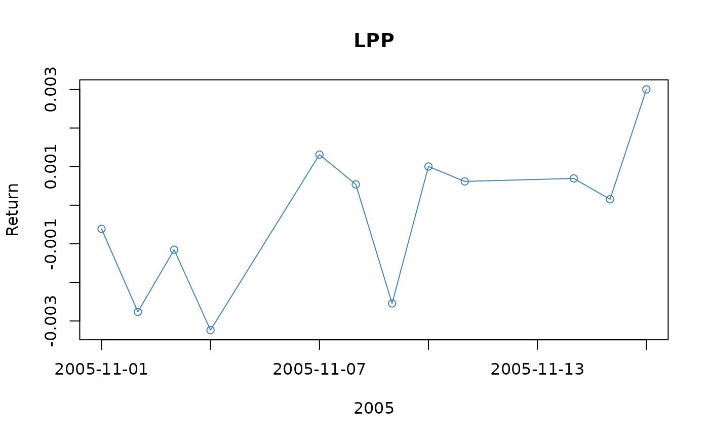
plot(LPP[, 1], at="auto", type = "o", col = "steelblue",
  main = "LPP", xlab = "2005", ylab = "Return")


## Example Plot 2
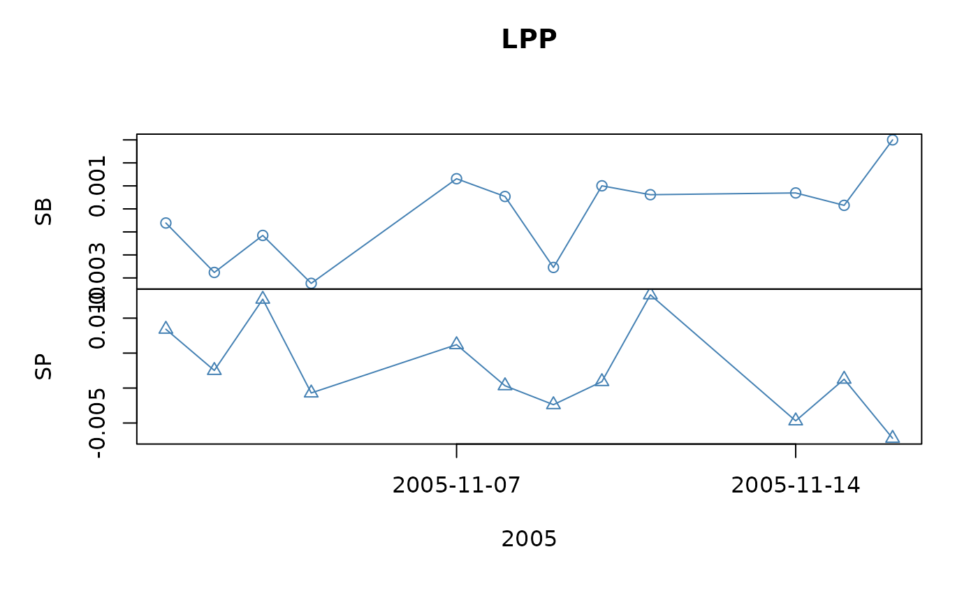
plot(LPP[, 1:2], type = "o", col = "steelblue",
  main = "LPP", xlab = "2005", ylab = "Return")


## Example Plot 3
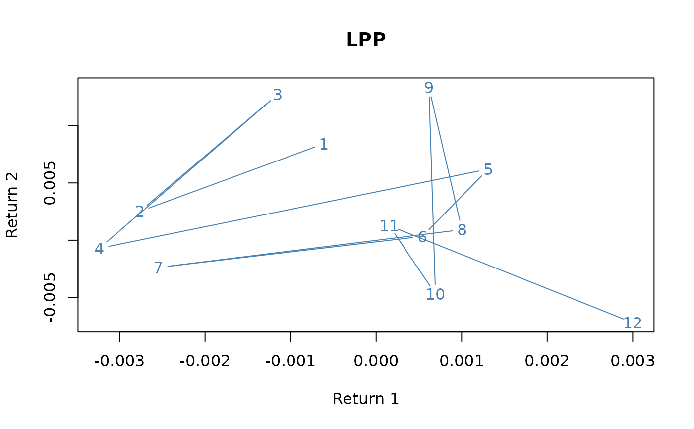
plot(LPP[, 1], LPP[, 2], type = "p", col = "steelblue",
  main = "LPP", xlab = "Return 1", ylab = "Return 2")


## Example Plot 4a, the wrong way to do it!
LPP <- as.timeSeries(data(LPP2005REC))
ZRH <- as.timeSeries(LPP[,"SPI"], zone = "Zurich", FinCenter = "Zurich")
NYC <- as.timeSeries(LPP[,"LMI"], zone = "NewYork", FinCenter = "NewYork")
finCenter(ZRH)
#> [1] "Zurich"
finCenter(NYC)
#> [1] "NewYork"
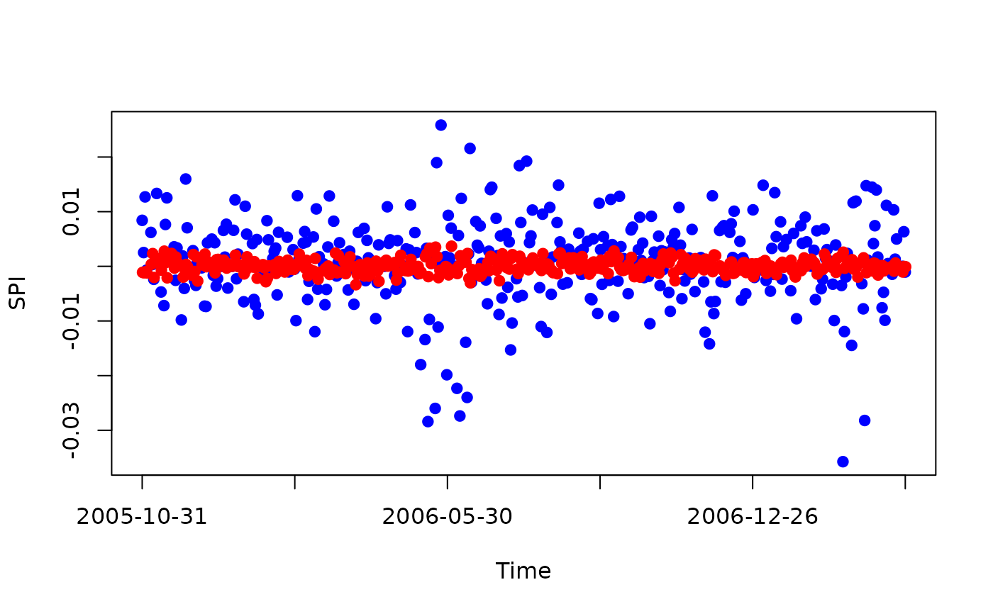
plot(ZRH, at="auto", type = "p", pch = 19, col = "blue")
points(NYC, pch = 19, col = "red")


## Example Plot 4b, convert NYC to Zurich time
finCenter(ZRH) <- "Zurich"
finCenter(NYC) <- "Zurich"
at <- unique(round(time(ZRH)))
plot(ZRH, type = "p", pch = 19, col = "blue", format = "%b %d", at = at,
    xlab = paste(ZRH@FinCenter, "local Time"), main = ZRH@FinCenter)
points(NYC, pch = 19, col = "red")


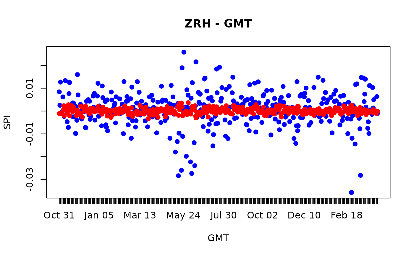
## Example 4c, force everything to GMT using "FinCenter" argument
finCenter(ZRH) <- "Zurich"
finCenter(NYC) <- "NewYork"
at <- unique(round(time(ZRH)))
plot(ZRH, type = "p", pch = 19, col = "blue", format = "%b %d", at = at,
    FinCenter = "GMT", xlab = "GMT", main = "ZRH - GMT")
points(NYC, FinCenter = "GMT", pch = 19, col = "red")