Bivariate Linear Interpolation

Bivariate Linear Interpolation. Options are available for gridded and pointwise interpolation.

Usage

linearInterp(x, y = NULL, z = NULL, gridPoints = 21,
    xo = seq(min(x), max(x), length = gridPoints),
    yo = seq(min(y), max(y), length = gridPoints))
    
linearInterpp(x, y = NULL, z = NULL, xo, yo)

Arguments

x, y, z

for linearInterp the arguments x and y are two numeric vectors of grid pounts, and z is a numeric matrix or any other rectangular object which can be transformed by the function as.matrix into a matrix object. For linearInterpp we consider either three numeric vectors of equal length or if y and z are NULL, a list with entries x, y, z, or named data frame with x in the first, y in the second, and z in the third column.

gridPoints

an integer value specifying the number of grid points in x and y direction.

xo, yo

for linearInterp two numeric vectors of data points spanning the grid, and for linearInterpp two numeric vectors of data points building pairs for pointwise interpolation.

Value

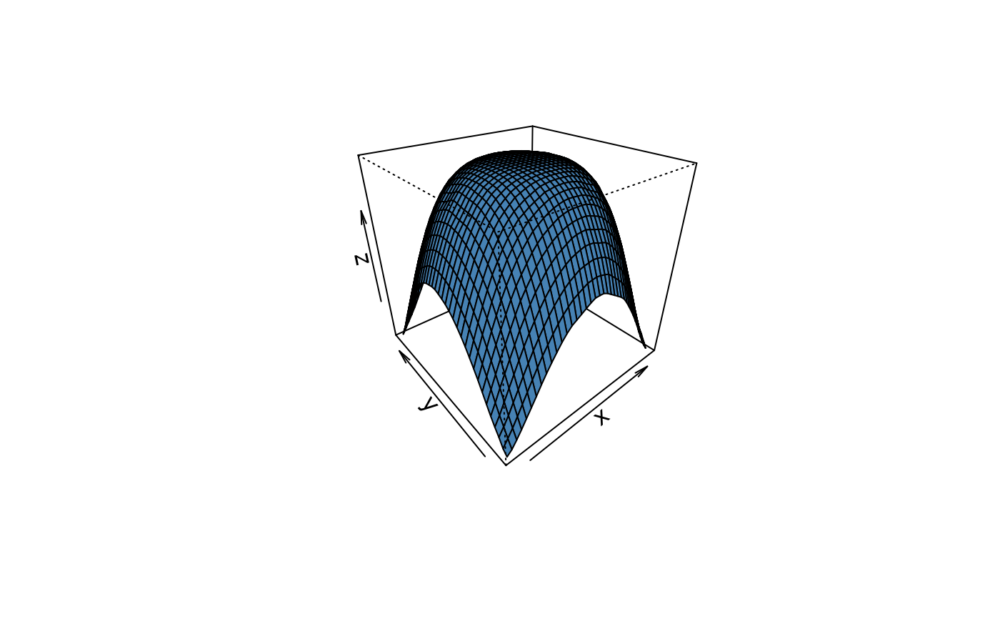
for linearInterp, a list with at least three entries, x, y and z. The returned values, can be used directly in persp and contour 3D plotting methods.

for linearInterpp, a data.frame with columns "x", "y", and "z".

See also

akimaInterp and krigeInterp

Examples

## Linear Interpolation:    
if (requireNamespace("interp")) {
    set.seed(1953)
    x <- runif(999) - 0.5
    y <- runif(999) - 0.5
    z <- cos(2 * pi * (x^2 + y^2))
    ans = linearInterp(x, y, z, gridPoints = 41)
    persp(ans, theta = -40, phi = 30, col = "steelblue",
          xlab = "x", ylab = "y", zlab = "z")
    contour(ans)
}