Standardized generalized error distribution

Functions to compute density, distribution function, quantile function and to generate random variates for the standardized generalized error distribution.

Usage

dged(x, mean = 0, sd = 1, nu = 2, log = FALSE)
pged(q, mean = 0, sd = 1, nu = 2)
qged(p, mean = 0, sd = 1, nu = 2)
rged(n, mean = 0, sd = 1, nu = 2)

Arguments

x, q

a numeric vector of quantiles.

p

a numeric vector of probabilities.

n

number of observations to simulate.

mean

location parameter.

sd

scale parameter.

nu

shape parameter.

log

logical; if TRUE, densities are given as log densities.

Details

The standardized GED is defined so that for a given sd it has the same variance, sd^2, for all values of the shape parameter, see the reference by Wuertz et al below.

dged computes the density, pged the distribution function, qged the quantile function, and rged generates random deviates from the standardized-t distribution with the specified parameters.

Value

numeric vector

References

Nelson D.B. (1991); Conditional Heteroscedasticity in Asset Returns: A New Approach, Econometrica, 59, 347–370.

Fernandez C., Steel M.F.J. (2000); On Bayesian Modelling of Fat Tails and Skewness, Preprint, 31 pages.

Wuertz D., Chalabi Y. and Luksan L. (????); Parameter estimation of ARMA models with GARCH/APARCH errors: An R and SPlus software implementation, Preprint, 41 pages, https://github.com/GeoBosh/fGarchDoc/blob/master/WurtzEtAlGarch.pdf

Author

Diethelm Wuertz for the Rmetrics R-port

See also

gedFit, absMoments, sged (skew GED),

gedSlider for visualization

Examples

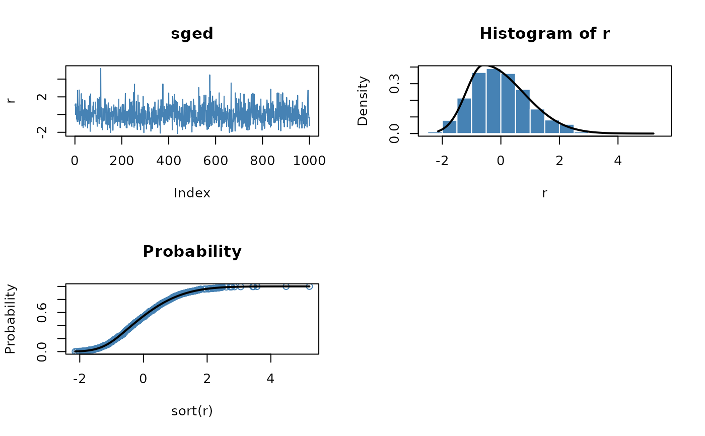
## sged -
   par(mfrow = c(2, 2))
   set.seed(1953)
   r = rsged(n = 1000)
   plot(r, type = "l", main = "sged", col = "steelblue")
   
   # Plot empirical density and compare with true density:
   hist(r, n = 25, probability = TRUE, border = "white", col = "steelblue")
   box()
   x = seq(min(r), max(r), length = 201)
   lines(x, dsged(x), lwd = 2)
   
   # Plot df and compare with true df:
   plot(sort(r), (1:1000/1000), main = "Probability", col = "steelblue",
     ylab = "Probability")
   lines(x, psged(x), lwd = 2)
   
   # Compute quantiles:
   round(qsged(psged(q = seq(-1, 5, by = 1))), digits = 6)
#> [1] -1  0  1  2  3  4  5