GARCH plot methods

Plot methods for GARCH modelling.

Usage

# S4 method for fGARCH,missing
plot(x, which = "ask", ...)

Arguments

x

an object of class "fGARCH".

which

a character string or a vector of positive integers specifying which plot(s) should be displayed, see section ‘Details’.

...

optional arguments to be passed.

Details

The plot method for "fGARCH" objects offers a selection of diagnostic, exploratory, and presentation plots from a menu. Argument which can be used to request specific plots. This is particularly useful in scripts.

If which is of length larger than one, all requested plots are produced. For this to be useful, the graphics window should be split beforehand in subwindows, e.g., using par(mfrow = ...), par(mfcol = ...), or layout() (see section ‘Examples’). If this is not done, then only the last plot will be visible.

The following graphs are available:

1	Time SeriesPlot
2	Conditional Standard Deviation Plot
3	Series Plot with 2 Conditional SD Superimposed
4	Autocorrelation function Plot of Observations
5	Autocorrelation function Plot of Squared Observations
6	Cross Correlation Plot
7	Residuals Plot
8	Conditional Standard Deviations Plot
9	Standardized Residuals Plot
10	ACF Plot of Standardized Residuals
11	ACF Plot of Squared Standardized Residuals
12	Cross Correlation Plot between $r^2$ and r
13	Quantile-Quantile Plot of Standardized Residuals
14	Series with -VaR Superimposed
15	Series with -ES Superimposed
16	Series with -VaR & -ES Superimposed

Author

Diethelm Wuertz for the Rmetrics R-port;

VaR and ES graphs were added by Georgi N. Boshnakov in v4033.92

See also

fGARCH method for tsdiag,

garchFit, class fGARCH,

predict, fitted, residuals VaR ES

plot

Examples

## simulate a Garch(1,1) time series
x <- garchSim(n = 200)
head(x) 
#> GMT 
#>                   garch
#> 2023-09-08  0.007522375
#> 2023-09-09 -0.001628817
#> 2023-09-10  0.003737262
#> 2023-09-11  0.004705047
#> 2023-09-12  0.001966999
#> 2023-09-13 -0.005850769

## fit GARCH(1,1) model
fit <- garchFit(formula = ~ garch(1, 1), data = x, trace = FALSE)

if (FALSE) {
## choose plots interactively
plot(fit)
}
   
## Batch Plot:
plot(fit, which = 3)

## a 2 by 2 matrix of plots
op <- par(mfrow = c(2,2))          # prepare 2x2 window
plot(fit, which = c(10, 11, 3, 16)) # plot

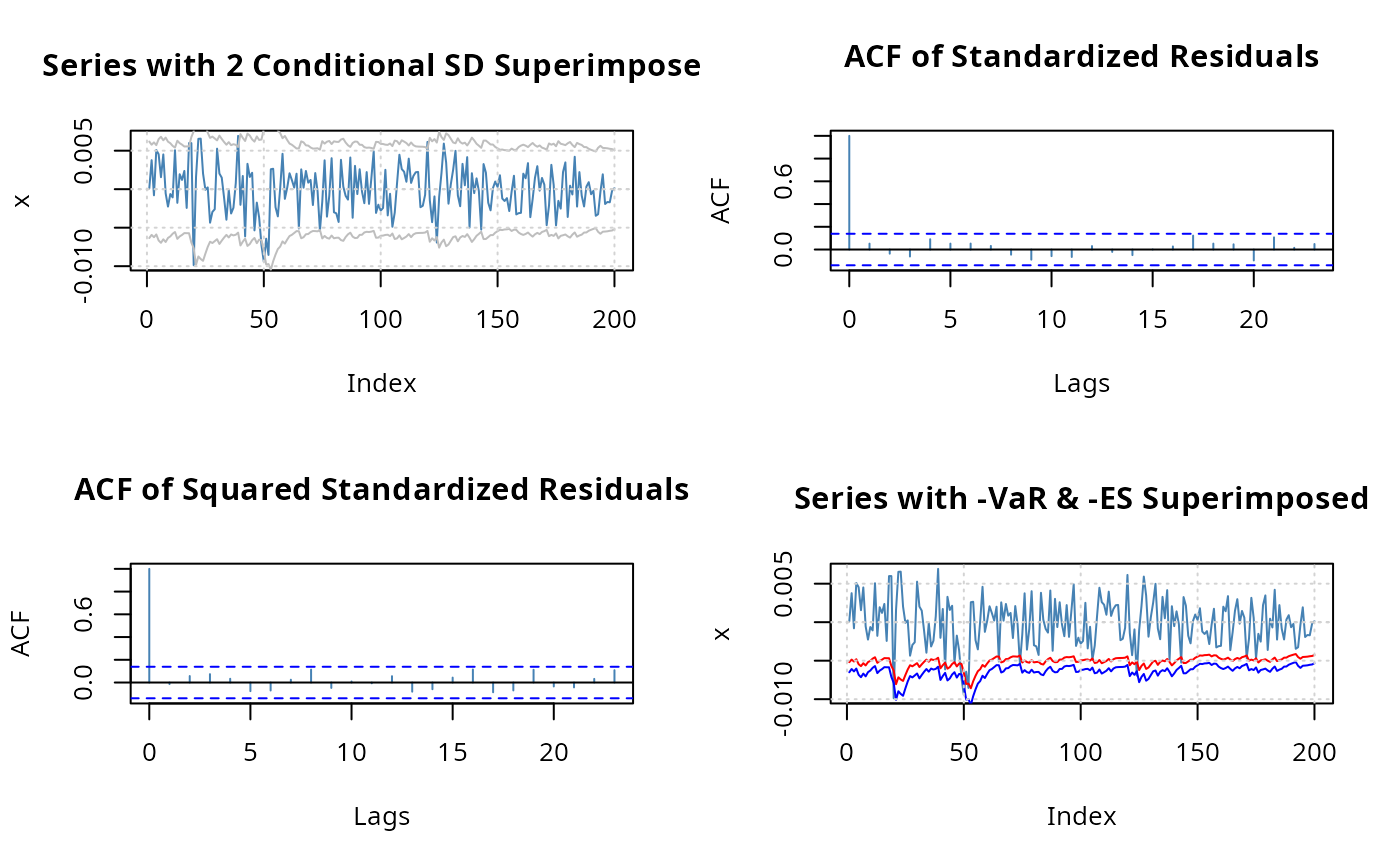par(op)                            # restore the previous layout