Skew Student-t distribution

Functions to compute density, distribution function, quantile function and to generate random variates for the skew Student-t distribution. Note that there are different ways to define a skew-t distribution, check section Details to see if this is the distribution you want.

Usage

dsstd(x, mean = 0, sd = 1, nu = 5, xi = 1.5, log = FALSE)
psstd(q, mean = 0, sd = 1, nu = 5, xi = 1.5)
qsstd(p, mean = 0, sd = 1, nu = 5, xi = 1.5)
rsstd(n, mean = 0, sd = 1, nu = 5, xi = 1.5)

Arguments

x, q

a numeric vector of quantiles.

p

a numeric vector of probabilities.

n

number of observations to simulate.

mean

location parameter.

sd

scale parameter.

nu

shape parameter (degrees of freedom).

xi

skewness parameter, a positive number. xi = 1 gives a symmetric distribution (here normal).

log

logical; if TRUE, densities are given as log densities.

Details

Skewness is based on the scheme by Fernandez and Steel (2000) but with different parameterisation as discussed by Wuertz et al (????), in that the skewness (xi), degrees of freedom (nu), mean (mean) and standard deviation (sd) are independent parameters.

dsstd computes the density, psstd the distribution function, qsstd the quantile function, and rsstd generates random deviates.

Value

numeric vector

References

Fernandez C., Steel M.F.J. (2000); On Bayesian Modelling of Fat Tails and Skewness, Preprint, 31 pages.

Wuertz D., Chalabi Y. and Luksan L. (????); Parameter estimation of ARMA models with GARCH/APARCH errors: An R and SPlus software implementation, Preprint, 41 pages, https://github.com/GeoBosh/fGarchDoc/blob/master/WurtzEtAlGarch.pdf

Author

Diethelm Wuertz for the Rmetrics R-port

See also

sstdFit (fit), sstdSlider (visualize)

snorm (skew normal), sged (skew GED)

Examples

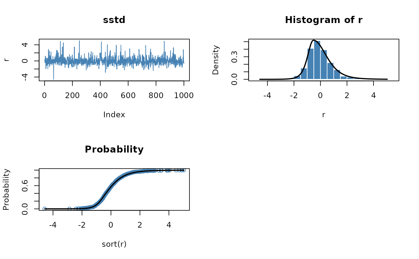
## sstd -
   par(mfrow = c(2, 2))
   set.seed(1953)
   r = rsstd(n = 1000)
   plot(r, type = "l", main = "sstd", col = "steelblue")
   
   # Plot empirical density and compare with true density:
   hist(r, n = 25, probability = TRUE, border = "white", col = "steelblue")
   box()
   x = seq(min(r), max(r), length = 201)
   lines(x, dsstd(x), lwd = 2)
   
   # Plot df and compare with true df:
   plot(sort(r), (1:1000/1000), main = "Probability", col = "steelblue",
     ylab = "Probability")
   lines(x, psstd(x), lwd = 2)
   
   # Compute quantiles:
   round(qsstd(psstd(q = seq(-1, 5, by = 1))), digits = 6)
#> [1] -1  0  1  2  3  4  5