Standardized Student-t distribution
dist-std.RdFunctions to compute density, distribution function, quantile function and to generate random variates for the standardized Student-t distribution.
Usage
dstd(x, mean = 0, sd = 1, nu = 5, log = FALSE)
pstd(q, mean = 0, sd = 1, nu = 5)
qstd(p, mean = 0, sd = 1, nu = 5)
rstd(n, mean = 0, sd = 1, nu = 5)Details
The standardized Student-t distribution is defined so that for a given
sd it has the same variance, sd^2, for all degrees of
freedom. For comparison, the variance of the usual Student-t
distribution is nu/(nu-2), where nu is the degrees of
freedom. The usual Student-t distribution is obtained by setting
sd = sqrt(nu/(nu - 2)).
Argument nu must be greater than 2. Although there is a default
value for nu, it is rather arbitrary and relying on it is
strongly discouraged.
dstd computes the density,
pstd the distribution function,
qstd the quantile function,
and
rstd generates random deviates from the standardized-t
distribution with the specified parameters.
References
Fernandez C., Steel M.F.J. (2000); On Bayesian Modelling of Fat Tails and Skewness, Preprint, 31 pages.
Wuertz D., Chalabi Y. and Luksan L. (2006); Parameter estimation of ARMA models with GARCH/APARCH errors: An R and SPlus software implementation, Preprint, 41 pages, https://github.com/GeoBosh/fGarchDoc/blob/master/WurtzEtAlGarch.pdf
Examples
## std -
pstd(1, sd = sqrt(5/(5-2)), nu = 5) == pt(1, df = 5) # TRUE
#> [1] TRUE
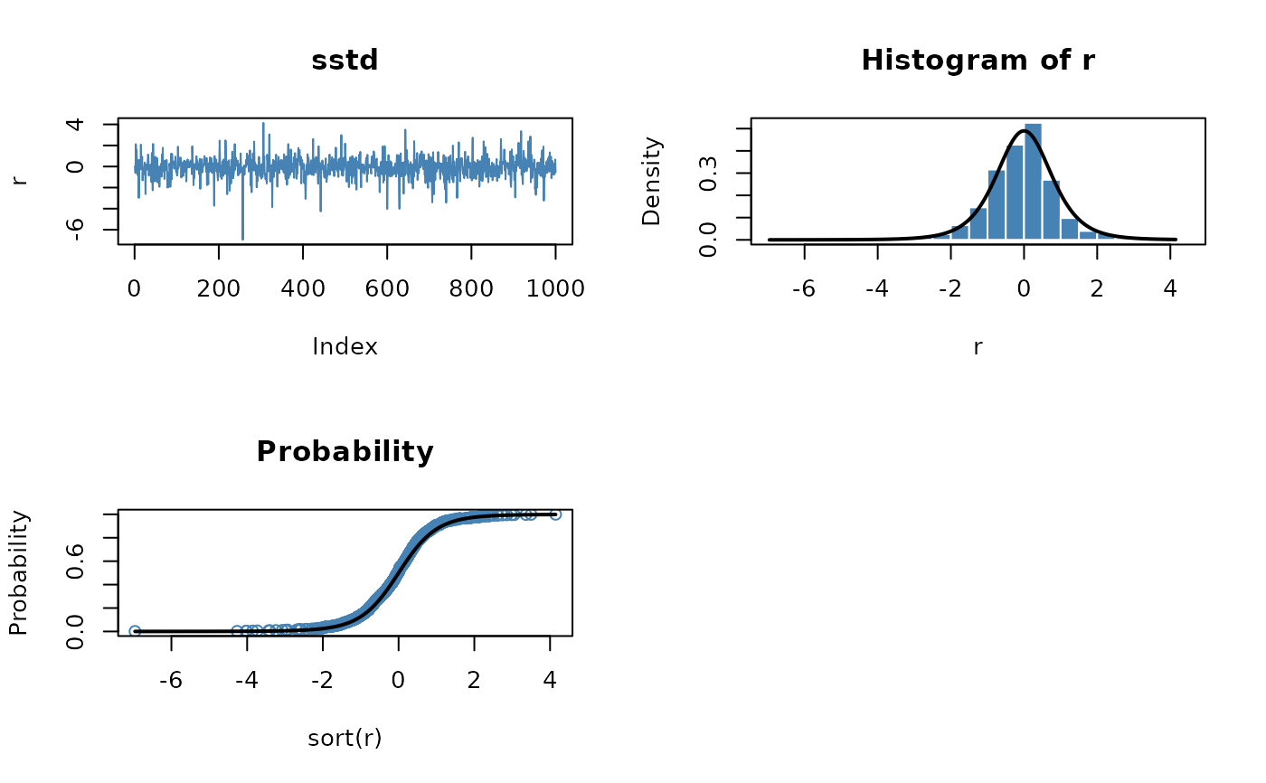
par(mfrow = c(2, 2))
set.seed(1953)
r = rstd(n = 1000)
plot(r, type = "l", main = "sstd", col = "steelblue")
# Plot empirical density and compare with true density:
hist(r, n = 25, probability = TRUE, border = "white", col = "steelblue")
box()
x = seq(min(r), max(r), length = 201)
lines(x, dstd(x), lwd = 2)
# Plot df and compare with true df:
plot(sort(r), (1:1000/1000), main = "Probability", col = "steelblue",
ylab = "Probability")
lines(x, pstd(x), lwd = 2)
# Compute quantiles:
round(qstd(pstd(q = seq(-1, 5, by = 1))), digits = 6)
#> [1] -1 0 1 2 3 4 5