Simulate from MixAR models

Usage

mixAR_sim(model, n, init, nskip = 100, flag = FALSE)

mixAny_sim(model, n, init, nskip=100, flag = FALSE,
                  theta, galpha0, galpha, gbeta)

Arguments

model: model from which to simulate, an object inheriting from class MixAR.
init: initial values, numeric vector.
n: size of the simulated series.
nskip: number of burn-in values, see Details.
flag: if TRUE return also the regimes.
theta: ma coef, a list.
galpha0: alpha0[k], k=1,...,g.
galpha: garch alpha.
gbeta: garch beta.

Details

mixAR_sim simulates a series of length nskip+n and returns the last n values.

mixAny_sim simulates from a MixAR model with GARCH innovations. mixAny_sim was a quick fix for Shahadat and needs consolidation.

The vector init provides the initial values for \(t=...,-1,0\). Its length must be at least equal to the maximal AR order. If it is longer, only the last max(model@order) elements are used.

Value

a numeric vector of length n. If flag = TRUE it has attribute regimes containing z.

Examples

exampleModels$WL_ibm
#> An object of class "MixARGaussian"
#> Number of components: 3 
#>        prob   shift scale   order ar_1   ar_2   
#> Comp_1 0.5439   0    4.8227   2   0.6792  0.3208
#> Comp_2 0.4176   0    6.0082   2   1.6711 -0.6711
#> Comp_3 0.0385   0   18.1716   1   1.0000        
#> 
#> Distributions of the error components:
#> 	standard Gaussian
#> 
## simulate a continuation of BJ ibm data
ts1 <- mixAR_sim(exampleModels$WL_ibm, n = 30, init = c(346, 352, 357), nskip = 0)

# a simulation based estimate of the 1-step predictive distribution
# for the first date after the data.
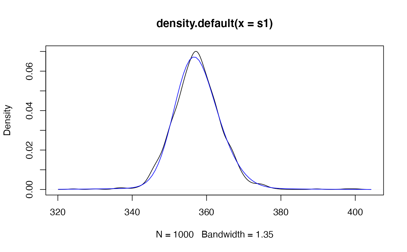
s1 <- replicate(1000, mixAR_sim(exampleModels$WL_ibm, n = 1, init = c(346, 352, 357), 
                      nskip = 0))
plot(density(s1))

# load ibm data from BJ
## data(ibmclose, package = "fma")

# overlay the 'true' predictive density.
pdf1 <- mix_pdf(exampleModels$WL_ibm, xcond = as.numeric(fma::ibmclose))
curve(pdf1, add = TRUE, col = 'blue')


# estimate of 5% quantile of predictive distribution
quantile(s1, 0.05)
#>       5% 
#> 347.3871 

# Monte Carlo estimate of "expected shortfall"
# (but the data has not been converted into returns...)
mean(s1[ s1 <= quantile(s1, 0.05) ])
#> [1] 344.1838