Example data from Franses (1996)

A multivariate time series containing the data used in examples by Franses (1996).

Usage

data("dataFranses1996")

Format

A multivariate quarterly time series.

Details

Each column is a quarterly time series. The time series start and end at different times, so NA's are used to align them in a single multivariate time series. Detailed account of the sources of the data is given by Franses (1996; Data Appendix, p. 214) .

year

(column 1)

The time formatted as yyyy.Q, where yyyy is the year and Q is the quarter (one of 1, 2, 3 or 4.). This column was part of the original data but is not really needed here since the time series object contains the time information.

USTotalIPI

(column 2)

Total Industrial Production Index for the United States (1985 = 100), 1960.1--1991.4.

CanadaUnemployment

(column 3)

Unemployment in Canada, measured in 1000 persons, 1960.1 - 1987.4.

GermanyGNP

(column 4)

Real GNP in Germany, 1960.1 - 1990.4 .

UKTotalInvestment

(column 5)

Real Total Investment in the United Kindom, 1955.1 - 1988.4.

SA_USTotalIPI

(column 6) Seasonally adjusted USTotalIPI.

SA_CanadaUnemployment

(column 7)

Seasonally adjusted CanadaUnemployment.

SA_GermanyGNP

(column 8)

Seasonally adjusted GermanyGNP.

UKGDP

(column 9)

United Kingdom gross domestic product (at 1985 prices), 1955.1--1988.4.

UKTotalConsumption

(column 10)

United Kingdom total consumption (at 1985 prices), 1955.1--1988.4.

UKNondurablesConsumption

(column 11)

United Kindom nondurables consumption (at 1985 prices), 1955.1--1988.4.

UKExport

(column 12)

United Kindom exports of goods and services (at 1985 prices), 1955.1--1988.4.

UKImport

(column 13)

United Kindom imports of goods and services (at 1985 prices), 1955.1--1988.4.

UKPublicInvestment

(column 14)

United Kindom public investment (at 1985 prices), 1962.1--1988.4.

UKWorkforce

(column 15)

United Kindom workforce (consisting of workforce in employment and unemployment), 1955.1--1988.4.

SwedenNondurablesConsumption

(column 16)

Real per capita non-durables consumption in Sweden (measured in logs), 1963.1--1988.1.

SwedenDisposableIncome

(column 17)

Real per capita disposable income in Sweden (measured in logs), 1963.1--1988.1.

SA_SwedenNondurablesConsumption

(column 18)

Seasonally adjusted SwedenNondurablesConsumption with Census X-11 method, 1964.1--1988.1. (Using the approximate linear Census X-11 filter given in Table 4.1, p. 52 in Franses (1996) and generating the forecasts and backcasts as described in Ooms (1994)).

SA_SwedenDisposableIncome

(column 19)

Seasonally adjusted SwedenDisposableIncome with Census X-11 method, 1964.1--1988.1. (Using the same method as above.)

More details on the individual time series are given by Franses (1996) .

Source

The data were downloaded from http://people.few.eur.nl/franses/research/data/data1.txt, but this link is now broken.

Note

Most of the time series in dataFranses1996 are available as separate datasets in package `partsm'. The numbers should be the same but note that, at the time of writing this, not all datasets there carry complete time information.

References

Franses PH (1996). Periodicity and Stochastic Trends In Economic Time Series. Oxford University Press Inc., New York.

Examples

data(dataFranses1996)
class(dataFranses1996)
#> [1] "mts"    "ts"     "matrix"
colnames(dataFranses1996)
#>  [1] "year"                            "USTotalIPI"                     
#>  [3] "CanadaUnemployment"              "GermanyGNP"                     
#>  [5] "UKTotalInvestment"               "SA_USTotalIPI"                  
#>  [7] "SA_CanadaUnemployment"           "SA_GermanyGNP"                  
#>  [9] "UKGDP"                           "UKTotalConsumption"             
#> [11] "UKNondurablesConsumption"        "UKExport"                       
#> [13] "UKImport"                        "UKPublicInvestment"             
#> [15] "UKWorkforce"                     "SwedenNondurablesConsumption"   
#> [17] "SwedenDisposableIncome"          "SA_SwedenNondurablesConsumption"
#> [19] "SA_SwedenDisposableIncome"      
dim(dataFranses1996) # c(148, 19)
#> [1] 148  19
plot(dataFranses1996[ , 2:11])


tipi <- dataFranses1996[ , "USTotalIPI"]
plot(tipi)

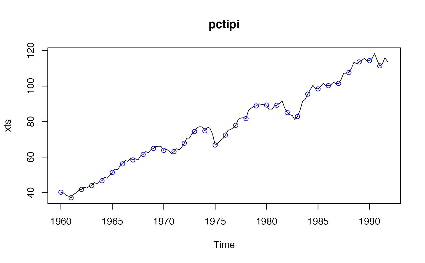
## convert to PeriodicTS and remove NA's at the start and end
pctipi <- pcts(tipi)
pctipi <- window(pctipi, start = availStart(pctipi), end = availEnd(pctipi))
plot(pctipi)


## convert  the whole dataset to class "PeriodicMTS"
pcfr <- pcts(dataFranses1996)

colnames(pcfr)[2:3] #  "USTotalIPI" "CanadaUnemployment"
#> [1] "USTotalIPI"         "CanadaUnemployment"

## subset as "PeriodicMTS"
pcfr2to3 <- pcfr[2:3]
plot(pcfr2to3)

## "[" "PeriodicMTS" even with length one arg.
pcfr2to2  <- pcfr[2]
pcfr2to2a <- pcfr["USTotalIPI"] # same

## use "[[" or $ to get "PeriodicTS"
pcfr2 <- pcfr[[2]]
pcfr2a <- pcfr[["USTotalIPI"]] # same
pcfr2b <- pcfr$USTotalIPI      # same
identical(pcfr2, pcfr2a) # TRUE
#> [1] TRUE
identical(pcfr2, pcfr2b) # TRUE
#> [1] TRUE

cycle(pcfr)
#> An object of class "PeriodicTS"
#> Slot "cycle": Start:  1955   Quarter_1 
#> Cycle:  QuarterYearCycle 
#> Number of seasons: 4 
#> 
#>       Q1 Q2 Q3 Q4
#> Y1955  1  2  3  4
#> Y1956  1  2  3  4
#> Y1957  1  2  3  4
#> Y1958  1  2  3  4
#> Y1959  1  2  3  4
#> Y1960  1  2  3  4
#> Y1961  1  2  3  4
#> Y1962  1  2  3  4
#> Y1963  1  2  3  4
#> Y1964  1  2  3  4
#> Y1965  1  2  3  4
#> Y1966  1  2  3  4
#> Y1967  1  2  3  4
#> Y1968  1  2  3  4
#> Y1969  1  2  3  4
#> Y1970  1  2  3  4
#> Y1971  1  2  3  4
#> Y1972  1  2  3  4
#> Y1973  1  2  3  4
#> Y1974  1  2  3  4
#> Y1975  1  2  3  4
#> Y1976  1  2  3  4
#> Y1977  1  2  3  4
#> Y1978  1  2  3  4
#> Y1979  1  2  3  4
#> Y1980  1  2  3  4
#> Y1981  1  2  3  4
#> Y1982  1  2  3  4
#> Y1983  1  2  3  4
#> Y1984  1  2  3  4
#> Y1985  1  2  3  4
#> Y1986  1  2  3  4
#> Y1987  1  2  3  4
#> Y1988  1  2  3  4
#> Y1989  1  2  3  4
#> Y1990  1  2  3  4
#> Y1991  1  2  3  4
frequency(pcfr)
#> [1] 4