The Kolmogorov Distribution

Compute the cdf of the Kolmogorov statistic for the two-sided test.

psi.pks(q, n, lower.tail = TRUE, log.p = FALSE, exact = NULL, warn = FALSE)

Arguments

q	vector of quantiles.
n	sample size.
lower.tail	logical; if TRUE (default) probabilities are P[X <= x], otherwise, P[X > x].
log.p	logical; if TRUE, probabilities p are given as log(p).
exact	if TRUE use exact method, if FALSE use asymptotic aproximation, if NULL (default) use exact method for n<=100 and asymptotic for n>100.
warn	logical; if TRUE (default) and exact=TRUE and n>100 print a message.

Details

Avoid setting exact=TRUE for large values of n since the exact method can become very slow for such n.

This function is a wrapper for two undocumented low level R functions which are used by ks.test.

Value

numerical vector of same length as q containing the values of the cdf of Kolmogorov's distribution.

References

See ks.test and, in the R sources, ks.c

See also

ks.test

Examples

xi <- seq(0,1,length=100)            # some x values

plot(xi,psi.pks(xi,4))               # cdf of D_4
lines(xi,psi.pks(xi,4))
lines(xi,psi.pks(xi,50),col="blue")  # overlay the cdf of  D_{50}
lines(xi,psi.pks(xi,100),col="red")  # overlay the cdf of  D_{100}
abline(h=0.95, col="brown")

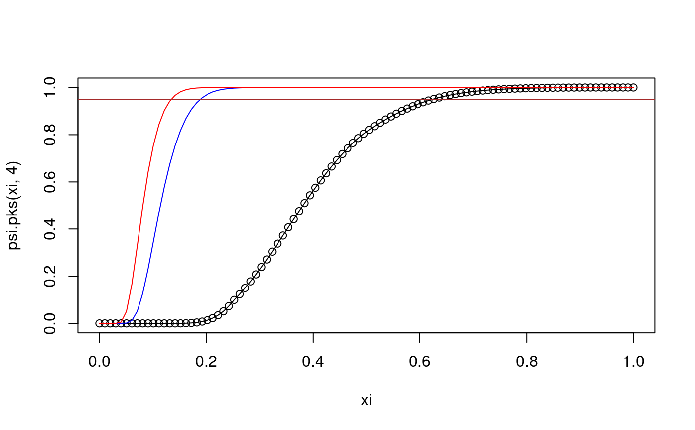
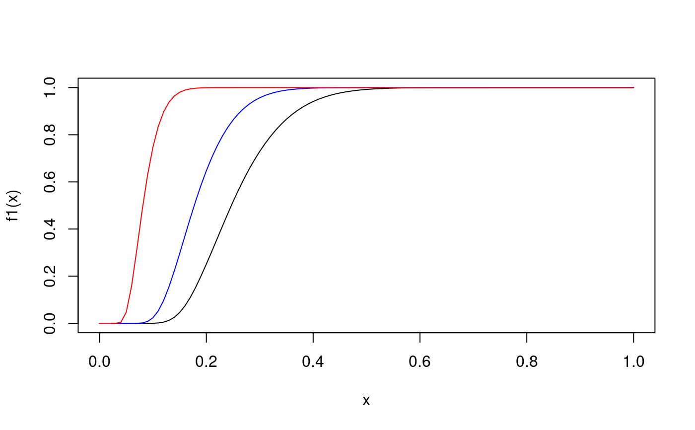
# q : P(Dn < q) = 0.95 for selected values of n
psi.pks(0.6239385,4)
#> [1] 0.95
psi.pks(0.2940753,20)
#> [1] 0.95
psi.pks(0.1340279,100)
#> [1] 0.95
psi.pks(0.04294685,1000)   # asymptotic approximation
#> [1] 0.95


n <- 8
plot(xi,psi.pks(xi,n,exact=FALSE))    # evaluate and plot asymptotic approx.
lines(xi,psi.pks(xi,n))               # overlay the exact cdf.

f1 <- function(x) psi.pks(x,10)      # f1(x) computes cdf of D_10
f2 <- function(x) psi.pks(x,20)      # f2(x) computes cdf of D_20
f3 <- function(x) psi.pks(x,100)     # f3(x) computes cdf of D_100

curve(f1,0,1)
curve(f2,0,1,add=TRUE,col="blue")
curve(f3,0,1,add=TRUE,col="red")