Forecasting functions for seasonal ARIMA models
fun.forecast.RdForecasting functions for seasonal ARIMA models.
Arguments
- past
past values of the time series, by default zeroes.
- n
number of forecasts to compute.
- eps
values of the white noise sequence (for simulation of future). Currently not used!
- pasteps
past values of the white noise sequence for models with MA terms, 0 by default.
- ...
specification of the model, passed to
new()to create a"SarimaModel"object, see Details.
Details
fun.forecast computes predictions from a SARIMA model. The
model is specified using the "..." arguments which are passed to
new("SarimaModel", ...), see the description of class
"SarimaModel" for details.
Argument past, if provided, should contain a least as many values as
needed for the prediction equation. It is harmless to provide more
values than necessary, even a whole time series.
fun.forecast can be used to illustrate, for example, the
inherent difference for prediction of integrated and seasonally
integrated models to corresponding models with roots close to the unit
circle.
Examples
f1 <- fun.forecast(past = 1, n = 100, ar = c(0.85), center = 5)
plot(f1)
 f2 <- fun.forecast(past = 8, n = 100, ar = c(0.85), center = 5)
plot(f2)
f2 <- fun.forecast(past = 8, n = 100, ar = c(0.85), center = 5)
plot(f2)
 f3 <- fun.forecast(past = 10, n = 100, ar = c(-0.85), center = 5)
plot(f3)
f3 <- fun.forecast(past = 10, n = 100, ar = c(-0.85), center = 5)
plot(f3)
 frw1 <- fun.forecast(past = 1, n = 100, iorder = 1)
plot(frw1)
frw1 <- fun.forecast(past = 1, n = 100, iorder = 1)
plot(frw1)
 frw2 <- fun.forecast(past = 3, n = 100, iorder = 1)
plot(frw2)
frw2 <- fun.forecast(past = 3, n = 100, iorder = 1)
plot(frw2)
 frwa1 <- fun.forecast(past = c(1, 2), n = 100, ar = c(0.85), iorder = 1)
plot(frwa1)
frwa1 <- fun.forecast(past = c(1, 2), n = 100, ar = c(0.85), iorder = 1)
plot(frwa1)
 fi2a <- fun.forecast(past = c(3, 1), n = 100, iorder = 2)
plot(fi2a)
fi2a <- fun.forecast(past = c(3, 1), n = 100, iorder = 2)
plot(fi2a)
 fi2b <- fun.forecast(past = c(1, 3), n = 100, iorder = 2)
plot(fi2b)
fi2b <- fun.forecast(past = c(1, 3), n = 100, iorder = 2)
plot(fi2b)
 fari1p2 <- fun.forecast(past = c(0, 1, 3), ar = c(0.9), n = 20, iorder = 2)
plot(fari1p2)
fari1p2 <- fun.forecast(past = c(0, 1, 3), ar = c(0.9), n = 20, iorder = 2)
plot(fari1p2)
 fsi1 <- fun.forecast(past = rnorm(4), n = 100, siorder = 1, nseasons = 4)
plot(fsi1)
fsi1 <- fun.forecast(past = rnorm(4), n = 100, siorder = 1, nseasons = 4)
plot(fsi1)
 fexa <- fun.forecast(past = rnorm(5), n = 100, ar = c(0.85), siorder = 1,
nseasons = 4)
plot(fexa)
fexa <- fun.forecast(past = rnorm(5), n = 100, ar = c(0.85), siorder = 1,
nseasons = 4)
plot(fexa)
 fi2a <- fun.forecast(past = rnorm(24, sd = 5), n = 120, siorder = 2,
nseasons = 12)
plot(fi2a)
fi2a <- fun.forecast(past = rnorm(24, sd = 5), n = 120, siorder = 2,
nseasons = 12)
plot(fi2a)
 fi1si1a <- fun.forecast(past = rnorm(24, sd = 5), n = 120, iorder = 1,
siorder = 1, nseasons = 12)
plot(fi1si1a)
fi1si1a <- fun.forecast(past = rnorm(24, sd = 5), n = 120, iorder = 1,
siorder = 1, nseasons = 12)
plot(fi1si1a)
 fi1si1a <- fun.forecast(past = AirPassengers[120:144], n = 120, iorder = 1,
siorder = 1, nseasons = 12)
plot(fi1si1a)
m1 <- list(iorder = 1, siorder = 1, ma = 0.8, nseasons = 12, sigma2 = 1)
m1
#> $iorder
#> [1] 1
#>
#> $siorder
#> [1] 1
#>
#> $ma
#> [1] 0.8
#>
#> $nseasons
#> [1] 12
#>
#> $sigma2
#> [1] 1
#>
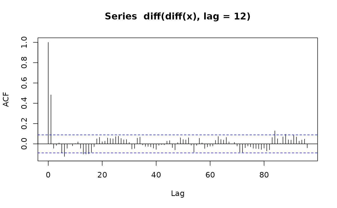
x <- sim_sarima(model = m1, n = 500)
acf(diff(diff(x), lag = 12), lag.max = 96)
fi1si1a <- fun.forecast(past = AirPassengers[120:144], n = 120, iorder = 1,
siorder = 1, nseasons = 12)
plot(fi1si1a)
m1 <- list(iorder = 1, siorder = 1, ma = 0.8, nseasons = 12, sigma2 = 1)
m1
#> $iorder
#> [1] 1
#>
#> $siorder
#> [1] 1
#>
#> $ma
#> [1] 0.8
#>
#> $nseasons
#> [1] 12
#>
#> $sigma2
#> [1] 1
#>
x <- sim_sarima(model = m1, n = 500)
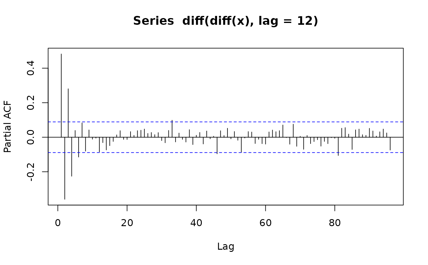
acf(diff(diff(x), lag = 12), lag.max = 96)
 pacf(diff(diff(x), lag = 12), lag.max = 96)
 m2 <- list(iorder = 1, siorder = 1, ma = 0.8, sma = 0.5, nseasons = 12,
sigma2 = 1)
m2
#> $iorder
#> [1] 1
#>
#> $siorder
#> [1] 1
#>
#> $ma
#> [1] 0.8
#>
#> $sma
#> [1] 0.5
#>
#> $nseasons
#> [1] 12
#>
#> $sigma2
#> [1] 1
#>
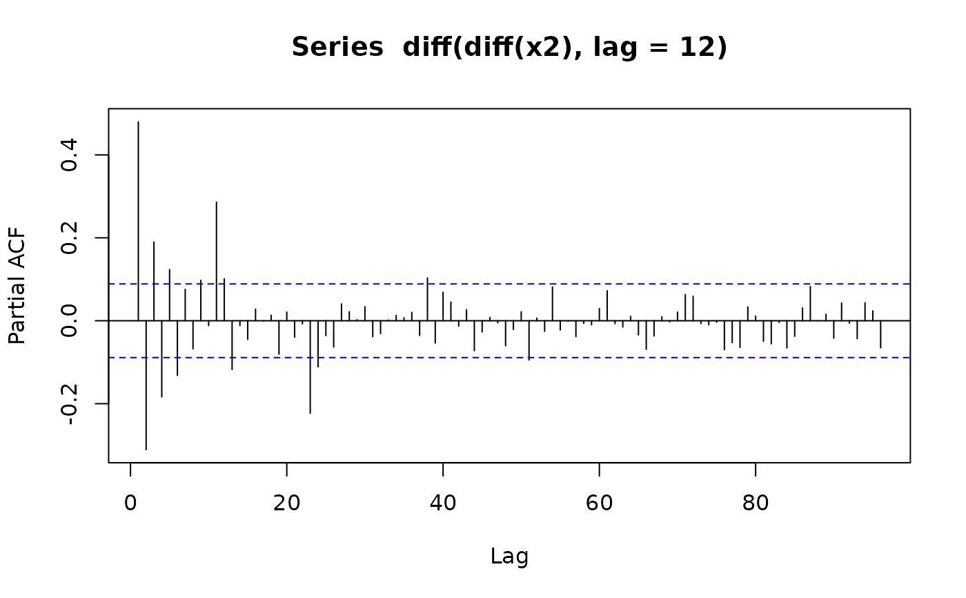
x2 <- sim_sarima(model = m2, n = 500)
acf(diff(diff(x2), lag = 12), lag.max = 96)
m2 <- list(iorder = 1, siorder = 1, ma = 0.8, sma = 0.5, nseasons = 12,
sigma2 = 1)
m2
#> $iorder
#> [1] 1
#>
#> $siorder
#> [1] 1
#>
#> $ma
#> [1] 0.8
#>
#> $sma
#> [1] 0.5
#>
#> $nseasons
#> [1] 12
#>
#> $sigma2
#> [1] 1
#>
x2 <- sim_sarima(model = m2, n = 500)
acf(diff(diff(x2), lag = 12), lag.max = 96)
 pacf(diff(diff(x2), lag = 12), lag.max = 96)
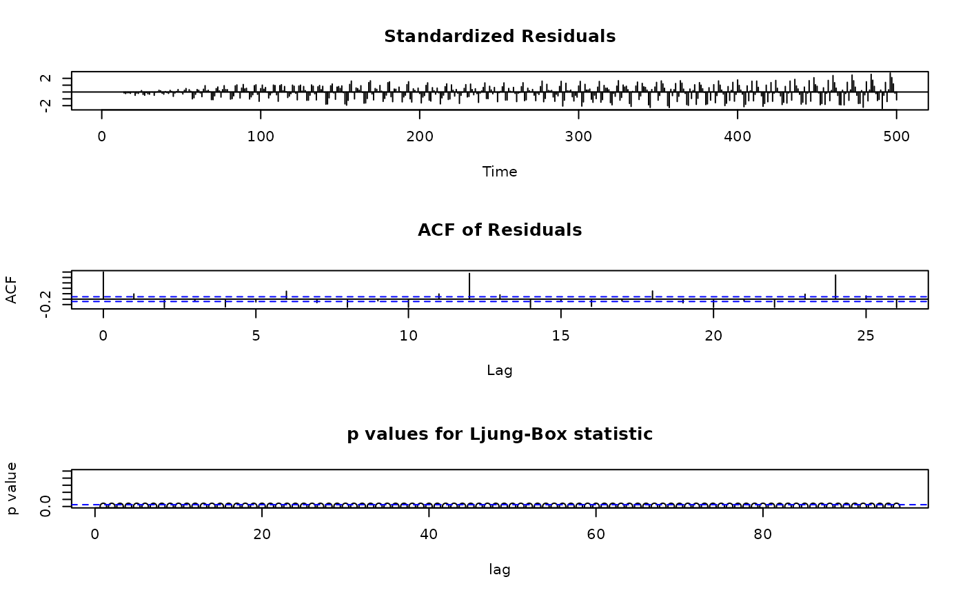
 fit2 <- arima(x2, order = c(0, 1, 1),
seasonal = list(order = c(0, 1, 0), nseasons = 12))
fit2
#>
#> Call:
#> arima(x = x2, order = c(0, 1, 1), seasonal = list(order = c(0, 1, 0), nseasons = 12))
#>
#> Coefficients:
#> ma1
#> -0.9844
#> s.e. 0.0058
#>
#> sigma^2 estimated as 38.83: log likelihood = -1619.52, aic = 3243.05
tsdiag(fit2)
fit2 <- arima(x2, order = c(0, 1, 1),
seasonal = list(order = c(0, 1, 0), nseasons = 12))
fit2
#>
#> Call:
#> arima(x = x2, order = c(0, 1, 1), seasonal = list(order = c(0, 1, 0), nseasons = 12))
#>
#> Coefficients:
#> ma1
#> -0.9844
#> s.e. 0.0058
#>
#> sigma^2 estimated as 38.83: log likelihood = -1619.52, aic = 3243.05
tsdiag(fit2)
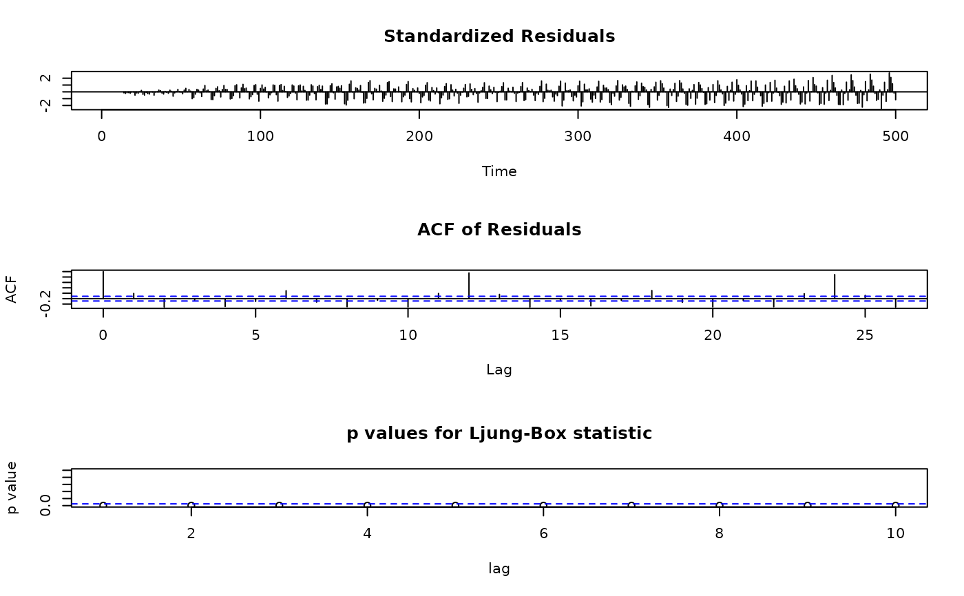 tsdiag(fit2, gof.lag = 96)
 x2past <- rnorm(13, sd = 10)
x2 <- sim_sarima(model = m2, n = 500, x = list(init = x2past))
plot(x2)
x2past <- rnorm(13, sd = 10)
x2 <- sim_sarima(model = m2, n = 500, x = list(init = x2past))
plot(x2)
 fun.forecast(ar = 0.5, n = 100)
#> Time Series:
#> Start = 1
#> End = 100
#> Frequency = 1
#> [1] 0 0 0 0 0 0 0 0 0 0 0 0 0 0 0 0 0 0 0 0 0 0 0 0 0 0 0 0 0 0 0 0 0 0 0 0 0
#> [38] 0 0 0 0 0 0 0 0 0 0 0 0 0 0 0 0 0 0 0 0 0 0 0 0 0 0 0 0 0 0 0 0 0 0 0 0 0
#> [75] 0 0 0 0 0 0 0 0 0 0 0 0 0 0 0 0 0 0 0 0 0 0 0 0 0 0
fun.forecast(ar = 0.5, n = 100, past = 1)
#> Time Series:
#> Start = 1
#> End = 100
#> Frequency = 1
#> [1] 5.000000e-01 2.500000e-01 1.250000e-01 6.250000e-02 3.125000e-02
#> [6] 1.562500e-02 7.812500e-03 3.906250e-03 1.953125e-03 9.765625e-04
#> [11] 4.882812e-04 2.441406e-04 1.220703e-04 6.103516e-05 3.051758e-05
#> [16] 1.525879e-05 7.629395e-06 3.814697e-06 1.907349e-06 9.536743e-07
#> [21] 4.768372e-07 2.384186e-07 1.192093e-07 5.960464e-08 2.980232e-08
#> [26] 1.490116e-08 7.450581e-09 3.725290e-09 1.862645e-09 9.313226e-10
#> [31] 4.656613e-10 2.328306e-10 1.164153e-10 5.820766e-11 2.910383e-11
#> [36] 1.455192e-11 7.275958e-12 3.637979e-12 1.818989e-12 9.094947e-13
#> [41] 4.547474e-13 2.273737e-13 1.136868e-13 5.684342e-14 2.842171e-14
#> [46] 1.421085e-14 7.105427e-15 3.552714e-15 1.776357e-15 8.881784e-16
#> [51] 4.440892e-16 2.220446e-16 1.110223e-16 5.551115e-17 2.775558e-17
#> [56] 1.387779e-17 6.938894e-18 3.469447e-18 1.734723e-18 8.673617e-19
#> [61] 4.336809e-19 2.168404e-19 1.084202e-19 5.421011e-20 2.710505e-20
#> [66] 1.355253e-20 6.776264e-21 3.388132e-21 1.694066e-21 8.470329e-22
#> [71] 4.235165e-22 2.117582e-22 1.058791e-22 5.293956e-23 2.646978e-23
#> [76] 1.323489e-23 6.617445e-24 3.308722e-24 1.654361e-24 8.271806e-25
#> [81] 4.135903e-25 2.067952e-25 1.033976e-25 5.169879e-26 2.584939e-26
#> [86] 1.292470e-26 6.462349e-27 3.231174e-27 1.615587e-27 8.077936e-28
#> [91] 4.038968e-28 2.019484e-28 1.009742e-28 5.048710e-29 2.524355e-29
#> [96] 1.262177e-29 6.310887e-30 3.155444e-30 1.577722e-30 7.888609e-31
fun.forecast(ma = 0.5, n = 100, past = 1)
#> Time Series:
#> Start = 1
#> End = 101
#> Frequency = 1
#> [1] 0 0 0 0 0 0 0 0 0 0 0 0 0 0 0 0 0 0 0 0 0 0 0 0 0 0 0 0 0 0 0 0 0 0 0 0 0
#> [38] 0 0 0 0 0 0 0 0 0 0 0 0 0 0 0 0 0 0 0 0 0 0 0 0 0 0 0 0 0 0 0 0 0 0 0 0 0
#> [75] 0 0 0 0 0 0 0 0 0 0 0 0 0 0 0 0 0 0 0 0 0 0 0 0 0 0 0
fun.forecast(iorder = 1, ma = 0.5, n = 100, past = 1)
#> Time Series:
#> Start = 1
#> End = 101
#> Frequency = 1
#> [1] 0 0 0 0 0 0 0 0 0 0 0 0 0 0 0 0 0 0 0 0 0 0 0 0 0 0 0 0 0 0 0 0 0 0 0 0 0
#> [38] 0 0 0 0 0 0 0 0 0 0 0 0 0 0 0 0 0 0 0 0 0 0 0 0 0 0 0 0 0 0 0 0 0 0 0 0 0
#> [75] 0 0 0 0 0 0 0 0 0 0 0 0 0 0 0 0 0 0 0 0 0 0 0 0 0 0 0
fun.forecast(iorder = 1, ma = 0.5, ar = 0.8, n = 100, past = 1)
#> Time Series:
#> Start = 1
#> End = 100
#> Frequency = 1
#> [1] 8.000000e-01 6.400000e-01 5.120000e-01 4.096000e-01 3.276800e-01
#> [6] 2.621440e-01 2.097152e-01 1.677722e-01 1.342177e-01 1.073742e-01
#> [11] 8.589935e-02 6.871948e-02 5.497558e-02 4.398047e-02 3.518437e-02
#> [16] 2.814750e-02 2.251800e-02 1.801440e-02 1.441152e-02 1.152922e-02
#> [21] 9.223372e-03 7.378698e-03 5.902958e-03 4.722366e-03 3.777893e-03
#> [26] 3.022315e-03 2.417852e-03 1.934281e-03 1.547425e-03 1.237940e-03
#> [31] 9.903520e-04 7.922816e-04 6.338253e-04 5.070602e-04 4.056482e-04
#> [36] 3.245186e-04 2.596148e-04 2.076919e-04 1.661535e-04 1.329228e-04
#> [41] 1.063382e-04 8.507059e-05 6.805647e-05 5.444518e-05 4.355614e-05
#> [46] 3.484491e-05 2.787593e-05 2.230075e-05 1.784060e-05 1.427248e-05
#> [51] 1.141798e-05 9.134385e-06 7.307508e-06 5.846007e-06 4.676805e-06
#> [56] 3.741444e-06 2.993155e-06 2.394524e-06 1.915619e-06 1.532496e-06
#> [61] 1.225996e-06 9.807971e-07 7.846377e-07 6.277102e-07 5.021681e-07
#> [66] 4.017345e-07 3.213876e-07 2.571101e-07 2.056881e-07 1.645505e-07
#> [71] 1.316404e-07 1.053123e-07 8.424983e-08 6.739987e-08 5.391989e-08
#> [76] 4.313591e-08 3.450873e-08 2.760699e-08 2.208559e-08 1.766847e-08
#> [81] 1.413478e-08 1.130782e-08 9.046257e-09 7.237006e-09 5.789604e-09
#> [86] 4.631684e-09 3.705347e-09 2.964277e-09 2.371422e-09 1.897138e-09
#> [91] 1.517710e-09 1.214168e-09 9.713344e-10 7.770676e-10 6.216540e-10
#> [96] 4.973232e-10 3.978586e-10 3.182869e-10 2.546295e-10 2.037036e-10
fun.forecast(m1, n = 100)
#> Time Series:
#> Start = 1
#> End = 101
#> Frequency = 1
#> $sigma2
#> [1] 0
#>
#> [[2]]
#> [1] 0
#>
#> [[3]]
#> [1] 0
#>
#> [[4]]
#> [1] 0
#>
#> [[5]]
#> [1] 0
#>
#> [[6]]
#> [1] 0
#>
#> [[7]]
#> [1] 0
#>
#> [[8]]
#> [1] 0
#>
#> [[9]]
#> [1] 0
#>
#> [[10]]
#> [1] 0
#>
#> [[11]]
#> [1] 0
#>
#> [[12]]
#> [1] 0
#>
#> [[13]]
#> [1] 0
#>
#> [[14]]
#> [1] 0
#>
#> [[15]]
#> [1] 0
#>
#> [[16]]
#> [1] 0
#>
#> [[17]]
#> [1] 0
#>
#> [[18]]
#> [1] 0
#>
#> [[19]]
#> [1] 0
#>
#> [[20]]
#> [1] 0
#>
#> [[21]]
#> [1] 0
#>
#> [[22]]
#> [1] 0
#>
#> [[23]]
#> [1] 0
#>
#> [[24]]
#> [1] 0
#>
#> [[25]]
#> [1] 0
#>
#> [[26]]
#> [1] 0
#>
#> [[27]]
#> [1] 0
#>
#> [[28]]
#> [1] 0
#>
#> [[29]]
#> [1] 0
#>
#> [[30]]
#> [1] 0
#>
#> [[31]]
#> [1] 0
#>
#> [[32]]
#> [1] 0
#>
#> [[33]]
#> [1] 0
#>
#> [[34]]
#> [1] 0
#>
#> [[35]]
#> [1] 0
#>
#> [[36]]
#> [1] 0
#>
#> [[37]]
#> [1] 0
#>
#> [[38]]
#> [1] 0
#>
#> [[39]]
#> [1] 0
#>
#> [[40]]
#> [1] 0
#>
#> [[41]]
#> [1] 0
#>
#> [[42]]
#> [1] 0
#>
#> [[43]]
#> [1] 0
#>
#> [[44]]
#> [1] 0
#>
#> [[45]]
#> [1] 0
#>
#> [[46]]
#> [1] 0
#>
#> [[47]]
#> [1] 0
#>
#> [[48]]
#> [1] 0
#>
#> [[49]]
#> [1] 0
#>
#> [[50]]
#> [1] 0
#>
#> [[51]]
#> [1] 0
#>
#> [[52]]
#> [1] 0
#>
#> [[53]]
#> [1] 0
#>
#> [[54]]
#> [1] 0
#>
#> [[55]]
#> [1] 0
#>
#> [[56]]
#> [1] 0
#>
#> [[57]]
#> [1] 0
#>
#> [[58]]
#> [1] 0
#>
#> [[59]]
#> [1] 0
#>
#> [[60]]
#> [1] 0
#>
#> [[61]]
#> [1] 0
#>
#> [[62]]
#> [1] 0
#>
#> [[63]]
#> [1] 0
#>
#> [[64]]
#> [1] 0
#>
#> [[65]]
#> [1] 0
#>
#> [[66]]
#> [1] 0
#>
#> [[67]]
#> [1] 0
#>
#> [[68]]
#> [1] 0
#>
#> [[69]]
#> [1] 0
#>
#> [[70]]
#> [1] 0
#>
#> [[71]]
#> [1] 0
#>
#> [[72]]
#> [1] 0
#>
#> [[73]]
#> [1] 0
#>
#> [[74]]
#> [1] 0
#>
#> [[75]]
#> [1] 0
#>
#> [[76]]
#> [1] 0
#>
#> [[77]]
#> [1] 0
#>
#> [[78]]
#> [1] 0
#>
#> [[79]]
#> [1] 0
#>
#> [[80]]
#> [1] 0
#>
#> [[81]]
#> [1] 0
#>
#> [[82]]
#> [1] 0
#>
#> [[83]]
#> [1] 0
#>
#> [[84]]
#> [1] 0
#>
#> [[85]]
#> [1] 0
#>
#> [[86]]
#> [1] 0
#>
#> [[87]]
#> [1] 0
#>
#> [[88]]
#> [1] 0
#>
#> [[89]]
#> [1] 0
#>
#> [[90]]
#> [1] 0
#>
#> [[91]]
#> [1] 0
#>
#> [[92]]
#> [1] 0
#>
#> [[93]]
#> [1] 0
#>
#> [[94]]
#> [1] 0
#>
#> [[95]]
#> [1] 0
#>
#> [[96]]
#> [1] 0
#>
#> [[97]]
#> [1] 0
#>
#> [[98]]
#> [1] 0
#>
#> [[99]]
#> [1] 0
#>
#> [[100]]
#> [1] 0
#>
#> [[101]]
#> [1] 0
#>
fun.forecast(m2, n = 100)
#> Time Series:
#> Start = 1
#> End = 101
#> Frequency = 1
#> $sigma2
#> [1] 0
#>
#> [[2]]
#> [1] 0
#>
#> [[3]]
#> [1] 0
#>
#> [[4]]
#> [1] 0
#>
#> [[5]]
#> [1] 0
#>
#> [[6]]
#> [1] 0
#>
#> [[7]]
#> [1] 0
#>
#> [[8]]
#> [1] 0
#>
#> [[9]]
#> [1] 0
#>
#> [[10]]
#> [1] 0
#>
#> [[11]]
#> [1] 0
#>
#> [[12]]
#> [1] 0
#>
#> [[13]]
#> [1] 0
#>
#> [[14]]
#> [1] 0
#>
#> [[15]]
#> [1] 0
#>
#> [[16]]
#> [1] 0
#>
#> [[17]]
#> [1] 0
#>
#> [[18]]
#> [1] 0
#>
#> [[19]]
#> [1] 0
#>
#> [[20]]
#> [1] 0
#>
#> [[21]]
#> [1] 0
#>
#> [[22]]
#> [1] 0
#>
#> [[23]]
#> [1] 0
#>
#> [[24]]
#> [1] 0
#>
#> [[25]]
#> [1] 0
#>
#> [[26]]
#> [1] 0
#>
#> [[27]]
#> [1] 0
#>
#> [[28]]
#> [1] 0
#>
#> [[29]]
#> [1] 0
#>
#> [[30]]
#> [1] 0
#>
#> [[31]]
#> [1] 0
#>
#> [[32]]
#> [1] 0
#>
#> [[33]]
#> [1] 0
#>
#> [[34]]
#> [1] 0
#>
#> [[35]]
#> [1] 0
#>
#> [[36]]
#> [1] 0
#>
#> [[37]]
#> [1] 0
#>
#> [[38]]
#> [1] 0
#>
#> [[39]]
#> [1] 0
#>
#> [[40]]
#> [1] 0
#>
#> [[41]]
#> [1] 0
#>
#> [[42]]
#> [1] 0
#>
#> [[43]]
#> [1] 0
#>
#> [[44]]
#> [1] 0
#>
#> [[45]]
#> [1] 0
#>
#> [[46]]
#> [1] 0
#>
#> [[47]]
#> [1] 0
#>
#> [[48]]
#> [1] 0
#>
#> [[49]]
#> [1] 0
#>
#> [[50]]
#> [1] 0
#>
#> [[51]]
#> [1] 0
#>
#> [[52]]
#> [1] 0
#>
#> [[53]]
#> [1] 0
#>
#> [[54]]
#> [1] 0
#>
#> [[55]]
#> [1] 0
#>
#> [[56]]
#> [1] 0
#>
#> [[57]]
#> [1] 0
#>
#> [[58]]
#> [1] 0
#>
#> [[59]]
#> [1] 0
#>
#> [[60]]
#> [1] 0
#>
#> [[61]]
#> [1] 0
#>
#> [[62]]
#> [1] 0
#>
#> [[63]]
#> [1] 0
#>
#> [[64]]
#> [1] 0
#>
#> [[65]]
#> [1] 0
#>
#> [[66]]
#> [1] 0
#>
#> [[67]]
#> [1] 0
#>
#> [[68]]
#> [1] 0
#>
#> [[69]]
#> [1] 0
#>
#> [[70]]
#> [1] 0
#>
#> [[71]]
#> [1] 0
#>
#> [[72]]
#> [1] 0
#>
#> [[73]]
#> [1] 0
#>
#> [[74]]
#> [1] 0
#>
#> [[75]]
#> [1] 0
#>
#> [[76]]
#> [1] 0
#>
#> [[77]]
#> [1] 0
#>
#> [[78]]
#> [1] 0
#>
#> [[79]]
#> [1] 0
#>
#> [[80]]
#> [1] 0
#>
#> [[81]]
#> [1] 0
#>
#> [[82]]
#> [1] 0
#>
#> [[83]]
#> [1] 0
#>
#> [[84]]
#> [1] 0
#>
#> [[85]]
#> [1] 0
#>
#> [[86]]
#> [1] 0
#>
#> [[87]]
#> [1] 0
#>
#> [[88]]
#> [1] 0
#>
#> [[89]]
#> [1] 0
#>
#> [[90]]
#> [1] 0
#>
#> [[91]]
#> [1] 0
#>
#> [[92]]
#> [1] 0
#>
#> [[93]]
#> [1] 0
#>
#> [[94]]
#> [1] 0
#>
#> [[95]]
#> [1] 0
#>
#> [[96]]
#> [1] 0
#>
#> [[97]]
#> [1] 0
#>
#> [[98]]
#> [1] 0
#>
#> [[99]]
#> [1] 0
#>
#> [[100]]
#> [1] 0
#>
#> [[101]]
#> [1] 0
#>
fun.forecast(iorder = 1, ar = 0.8, ma = 0.5, n = 100, past = 1)
#> Time Series:
#> Start = 1
#> End = 100
#> Frequency = 1
#> [1] 8.000000e-01 6.400000e-01 5.120000e-01 4.096000e-01 3.276800e-01
#> [6] 2.621440e-01 2.097152e-01 1.677722e-01 1.342177e-01 1.073742e-01
#> [11] 8.589935e-02 6.871948e-02 5.497558e-02 4.398047e-02 3.518437e-02
#> [16] 2.814750e-02 2.251800e-02 1.801440e-02 1.441152e-02 1.152922e-02
#> [21] 9.223372e-03 7.378698e-03 5.902958e-03 4.722366e-03 3.777893e-03
#> [26] 3.022315e-03 2.417852e-03 1.934281e-03 1.547425e-03 1.237940e-03
#> [31] 9.903520e-04 7.922816e-04 6.338253e-04 5.070602e-04 4.056482e-04
#> [36] 3.245186e-04 2.596148e-04 2.076919e-04 1.661535e-04 1.329228e-04
#> [41] 1.063382e-04 8.507059e-05 6.805647e-05 5.444518e-05 4.355614e-05
#> [46] 3.484491e-05 2.787593e-05 2.230075e-05 1.784060e-05 1.427248e-05
#> [51] 1.141798e-05 9.134385e-06 7.307508e-06 5.846007e-06 4.676805e-06
#> [56] 3.741444e-06 2.993155e-06 2.394524e-06 1.915619e-06 1.532496e-06
#> [61] 1.225996e-06 9.807971e-07 7.846377e-07 6.277102e-07 5.021681e-07
#> [66] 4.017345e-07 3.213876e-07 2.571101e-07 2.056881e-07 1.645505e-07
#> [71] 1.316404e-07 1.053123e-07 8.424983e-08 6.739987e-08 5.391989e-08
#> [76] 4.313591e-08 3.450873e-08 2.760699e-08 2.208559e-08 1.766847e-08
#> [81] 1.413478e-08 1.130782e-08 9.046257e-09 7.237006e-09 5.789604e-09
#> [86] 4.631684e-09 3.705347e-09 2.964277e-09 2.371422e-09 1.897138e-09
#> [91] 1.517710e-09 1.214168e-09 9.713344e-10 7.770676e-10 6.216540e-10
#> [96] 4.973232e-10 3.978586e-10 3.182869e-10 2.546295e-10 2.037036e-10
fun.forecast(ar = 0.5, n = 100)
#> Time Series:
#> Start = 1
#> End = 100
#> Frequency = 1
#> [1] 0 0 0 0 0 0 0 0 0 0 0 0 0 0 0 0 0 0 0 0 0 0 0 0 0 0 0 0 0 0 0 0 0 0 0 0 0
#> [38] 0 0 0 0 0 0 0 0 0 0 0 0 0 0 0 0 0 0 0 0 0 0 0 0 0 0 0 0 0 0 0 0 0 0 0 0 0
#> [75] 0 0 0 0 0 0 0 0 0 0 0 0 0 0 0 0 0 0 0 0 0 0 0 0 0 0
fun.forecast(ar = 0.5, n = 100, past = 1)
#> Time Series:
#> Start = 1
#> End = 100
#> Frequency = 1
#> [1] 5.000000e-01 2.500000e-01 1.250000e-01 6.250000e-02 3.125000e-02
#> [6] 1.562500e-02 7.812500e-03 3.906250e-03 1.953125e-03 9.765625e-04
#> [11] 4.882812e-04 2.441406e-04 1.220703e-04 6.103516e-05 3.051758e-05
#> [16] 1.525879e-05 7.629395e-06 3.814697e-06 1.907349e-06 9.536743e-07
#> [21] 4.768372e-07 2.384186e-07 1.192093e-07 5.960464e-08 2.980232e-08
#> [26] 1.490116e-08 7.450581e-09 3.725290e-09 1.862645e-09 9.313226e-10
#> [31] 4.656613e-10 2.328306e-10 1.164153e-10 5.820766e-11 2.910383e-11
#> [36] 1.455192e-11 7.275958e-12 3.637979e-12 1.818989e-12 9.094947e-13
#> [41] 4.547474e-13 2.273737e-13 1.136868e-13 5.684342e-14 2.842171e-14
#> [46] 1.421085e-14 7.105427e-15 3.552714e-15 1.776357e-15 8.881784e-16
#> [51] 4.440892e-16 2.220446e-16 1.110223e-16 5.551115e-17 2.775558e-17
#> [56] 1.387779e-17 6.938894e-18 3.469447e-18 1.734723e-18 8.673617e-19
#> [61] 4.336809e-19 2.168404e-19 1.084202e-19 5.421011e-20 2.710505e-20
#> [66] 1.355253e-20 6.776264e-21 3.388132e-21 1.694066e-21 8.470329e-22
#> [71] 4.235165e-22 2.117582e-22 1.058791e-22 5.293956e-23 2.646978e-23
#> [76] 1.323489e-23 6.617445e-24 3.308722e-24 1.654361e-24 8.271806e-25
#> [81] 4.135903e-25 2.067952e-25 1.033976e-25 5.169879e-26 2.584939e-26
#> [86] 1.292470e-26 6.462349e-27 3.231174e-27 1.615587e-27 8.077936e-28
#> [91] 4.038968e-28 2.019484e-28 1.009742e-28 5.048710e-29 2.524355e-29
#> [96] 1.262177e-29 6.310887e-30 3.155444e-30 1.577722e-30 7.888609e-31
fun.forecast(ma = 0.5, n = 100, past = 1)
#> Time Series:
#> Start = 1
#> End = 101
#> Frequency = 1
#> [1] 0 0 0 0 0 0 0 0 0 0 0 0 0 0 0 0 0 0 0 0 0 0 0 0 0 0 0 0 0 0 0 0 0 0 0 0 0
#> [38] 0 0 0 0 0 0 0 0 0 0 0 0 0 0 0 0 0 0 0 0 0 0 0 0 0 0 0 0 0 0 0 0 0 0 0 0 0
#> [75] 0 0 0 0 0 0 0 0 0 0 0 0 0 0 0 0 0 0 0 0 0 0 0 0 0 0 0
fun.forecast(iorder = 1, ma = 0.5, n = 100, past = 1)
#> Time Series:
#> Start = 1
#> End = 101
#> Frequency = 1
#> [1] 0 0 0 0 0 0 0 0 0 0 0 0 0 0 0 0 0 0 0 0 0 0 0 0 0 0 0 0 0 0 0 0 0 0 0 0 0
#> [38] 0 0 0 0 0 0 0 0 0 0 0 0 0 0 0 0 0 0 0 0 0 0 0 0 0 0 0 0 0 0 0 0 0 0 0 0 0
#> [75] 0 0 0 0 0 0 0 0 0 0 0 0 0 0 0 0 0 0 0 0 0 0 0 0 0 0 0
fun.forecast(iorder = 1, ma = 0.5, ar = 0.8, n = 100, past = 1)
#> Time Series:
#> Start = 1
#> End = 100
#> Frequency = 1
#> [1] 8.000000e-01 6.400000e-01 5.120000e-01 4.096000e-01 3.276800e-01
#> [6] 2.621440e-01 2.097152e-01 1.677722e-01 1.342177e-01 1.073742e-01
#> [11] 8.589935e-02 6.871948e-02 5.497558e-02 4.398047e-02 3.518437e-02
#> [16] 2.814750e-02 2.251800e-02 1.801440e-02 1.441152e-02 1.152922e-02
#> [21] 9.223372e-03 7.378698e-03 5.902958e-03 4.722366e-03 3.777893e-03
#> [26] 3.022315e-03 2.417852e-03 1.934281e-03 1.547425e-03 1.237940e-03
#> [31] 9.903520e-04 7.922816e-04 6.338253e-04 5.070602e-04 4.056482e-04
#> [36] 3.245186e-04 2.596148e-04 2.076919e-04 1.661535e-04 1.329228e-04
#> [41] 1.063382e-04 8.507059e-05 6.805647e-05 5.444518e-05 4.355614e-05
#> [46] 3.484491e-05 2.787593e-05 2.230075e-05 1.784060e-05 1.427248e-05
#> [51] 1.141798e-05 9.134385e-06 7.307508e-06 5.846007e-06 4.676805e-06
#> [56] 3.741444e-06 2.993155e-06 2.394524e-06 1.915619e-06 1.532496e-06
#> [61] 1.225996e-06 9.807971e-07 7.846377e-07 6.277102e-07 5.021681e-07
#> [66] 4.017345e-07 3.213876e-07 2.571101e-07 2.056881e-07 1.645505e-07
#> [71] 1.316404e-07 1.053123e-07 8.424983e-08 6.739987e-08 5.391989e-08
#> [76] 4.313591e-08 3.450873e-08 2.760699e-08 2.208559e-08 1.766847e-08
#> [81] 1.413478e-08 1.130782e-08 9.046257e-09 7.237006e-09 5.789604e-09
#> [86] 4.631684e-09 3.705347e-09 2.964277e-09 2.371422e-09 1.897138e-09
#> [91] 1.517710e-09 1.214168e-09 9.713344e-10 7.770676e-10 6.216540e-10
#> [96] 4.973232e-10 3.978586e-10 3.182869e-10 2.546295e-10 2.037036e-10
fun.forecast(m1, n = 100)
#> Time Series:
#> Start = 1
#> End = 101
#> Frequency = 1
#> $sigma2
#> [1] 0
#>
#> [[2]]
#> [1] 0
#>
#> [[3]]
#> [1] 0
#>
#> [[4]]
#> [1] 0
#>
#> [[5]]
#> [1] 0
#>
#> [[6]]
#> [1] 0
#>
#> [[7]]
#> [1] 0
#>
#> [[8]]
#> [1] 0
#>
#> [[9]]
#> [1] 0
#>
#> [[10]]
#> [1] 0
#>
#> [[11]]
#> [1] 0
#>
#> [[12]]
#> [1] 0
#>
#> [[13]]
#> [1] 0
#>
#> [[14]]
#> [1] 0
#>
#> [[15]]
#> [1] 0
#>
#> [[16]]
#> [1] 0
#>
#> [[17]]
#> [1] 0
#>
#> [[18]]
#> [1] 0
#>
#> [[19]]
#> [1] 0
#>
#> [[20]]
#> [1] 0
#>
#> [[21]]
#> [1] 0
#>
#> [[22]]
#> [1] 0
#>
#> [[23]]
#> [1] 0
#>
#> [[24]]
#> [1] 0
#>
#> [[25]]
#> [1] 0
#>
#> [[26]]
#> [1] 0
#>
#> [[27]]
#> [1] 0
#>
#> [[28]]
#> [1] 0
#>
#> [[29]]
#> [1] 0
#>
#> [[30]]
#> [1] 0
#>
#> [[31]]
#> [1] 0
#>
#> [[32]]
#> [1] 0
#>
#> [[33]]
#> [1] 0
#>
#> [[34]]
#> [1] 0
#>
#> [[35]]
#> [1] 0
#>
#> [[36]]
#> [1] 0
#>
#> [[37]]
#> [1] 0
#>
#> [[38]]
#> [1] 0
#>
#> [[39]]
#> [1] 0
#>
#> [[40]]
#> [1] 0
#>
#> [[41]]
#> [1] 0
#>
#> [[42]]
#> [1] 0
#>
#> [[43]]
#> [1] 0
#>
#> [[44]]
#> [1] 0
#>
#> [[45]]
#> [1] 0
#>
#> [[46]]
#> [1] 0
#>
#> [[47]]
#> [1] 0
#>
#> [[48]]
#> [1] 0
#>
#> [[49]]
#> [1] 0
#>
#> [[50]]
#> [1] 0
#>
#> [[51]]
#> [1] 0
#>
#> [[52]]
#> [1] 0
#>
#> [[53]]
#> [1] 0
#>
#> [[54]]
#> [1] 0
#>
#> [[55]]
#> [1] 0
#>
#> [[56]]
#> [1] 0
#>
#> [[57]]
#> [1] 0
#>
#> [[58]]
#> [1] 0
#>
#> [[59]]
#> [1] 0
#>
#> [[60]]
#> [1] 0
#>
#> [[61]]
#> [1] 0
#>
#> [[62]]
#> [1] 0
#>
#> [[63]]
#> [1] 0
#>
#> [[64]]
#> [1] 0
#>
#> [[65]]
#> [1] 0
#>
#> [[66]]
#> [1] 0
#>
#> [[67]]
#> [1] 0
#>
#> [[68]]
#> [1] 0
#>
#> [[69]]
#> [1] 0
#>
#> [[70]]
#> [1] 0
#>
#> [[71]]
#> [1] 0
#>
#> [[72]]
#> [1] 0
#>
#> [[73]]
#> [1] 0
#>
#> [[74]]
#> [1] 0
#>
#> [[75]]
#> [1] 0
#>
#> [[76]]
#> [1] 0
#>
#> [[77]]
#> [1] 0
#>
#> [[78]]
#> [1] 0
#>
#> [[79]]
#> [1] 0
#>
#> [[80]]
#> [1] 0
#>
#> [[81]]
#> [1] 0
#>
#> [[82]]
#> [1] 0
#>
#> [[83]]
#> [1] 0
#>
#> [[84]]
#> [1] 0
#>
#> [[85]]
#> [1] 0
#>
#> [[86]]
#> [1] 0
#>
#> [[87]]
#> [1] 0
#>
#> [[88]]
#> [1] 0
#>
#> [[89]]
#> [1] 0
#>
#> [[90]]
#> [1] 0
#>
#> [[91]]
#> [1] 0
#>
#> [[92]]
#> [1] 0
#>
#> [[93]]
#> [1] 0
#>
#> [[94]]
#> [1] 0
#>
#> [[95]]
#> [1] 0
#>
#> [[96]]
#> [1] 0
#>
#> [[97]]
#> [1] 0
#>
#> [[98]]
#> [1] 0
#>
#> [[99]]
#> [1] 0
#>
#> [[100]]
#> [1] 0
#>
#> [[101]]
#> [1] 0
#>
fun.forecast(m2, n = 100)
#> Time Series:
#> Start = 1
#> End = 101
#> Frequency = 1
#> $sigma2
#> [1] 0
#>
#> [[2]]
#> [1] 0
#>
#> [[3]]
#> [1] 0
#>
#> [[4]]
#> [1] 0
#>
#> [[5]]
#> [1] 0
#>
#> [[6]]
#> [1] 0
#>
#> [[7]]
#> [1] 0
#>
#> [[8]]
#> [1] 0
#>
#> [[9]]
#> [1] 0
#>
#> [[10]]
#> [1] 0
#>
#> [[11]]
#> [1] 0
#>
#> [[12]]
#> [1] 0
#>
#> [[13]]
#> [1] 0
#>
#> [[14]]
#> [1] 0
#>
#> [[15]]
#> [1] 0
#>
#> [[16]]
#> [1] 0
#>
#> [[17]]
#> [1] 0
#>
#> [[18]]
#> [1] 0
#>
#> [[19]]
#> [1] 0
#>
#> [[20]]
#> [1] 0
#>
#> [[21]]
#> [1] 0
#>
#> [[22]]
#> [1] 0
#>
#> [[23]]
#> [1] 0
#>
#> [[24]]
#> [1] 0
#>
#> [[25]]
#> [1] 0
#>
#> [[26]]
#> [1] 0
#>
#> [[27]]
#> [1] 0
#>
#> [[28]]
#> [1] 0
#>
#> [[29]]
#> [1] 0
#>
#> [[30]]
#> [1] 0
#>
#> [[31]]
#> [1] 0
#>
#> [[32]]
#> [1] 0
#>
#> [[33]]
#> [1] 0
#>
#> [[34]]
#> [1] 0
#>
#> [[35]]
#> [1] 0
#>
#> [[36]]
#> [1] 0
#>
#> [[37]]
#> [1] 0
#>
#> [[38]]
#> [1] 0
#>
#> [[39]]
#> [1] 0
#>
#> [[40]]
#> [1] 0
#>
#> [[41]]
#> [1] 0
#>
#> [[42]]
#> [1] 0
#>
#> [[43]]
#> [1] 0
#>
#> [[44]]
#> [1] 0
#>
#> [[45]]
#> [1] 0
#>
#> [[46]]
#> [1] 0
#>
#> [[47]]
#> [1] 0
#>
#> [[48]]
#> [1] 0
#>
#> [[49]]
#> [1] 0
#>
#> [[50]]
#> [1] 0
#>
#> [[51]]
#> [1] 0
#>
#> [[52]]
#> [1] 0
#>
#> [[53]]
#> [1] 0
#>
#> [[54]]
#> [1] 0
#>
#> [[55]]
#> [1] 0
#>
#> [[56]]
#> [1] 0
#>
#> [[57]]
#> [1] 0
#>
#> [[58]]
#> [1] 0
#>
#> [[59]]
#> [1] 0
#>
#> [[60]]
#> [1] 0
#>
#> [[61]]
#> [1] 0
#>
#> [[62]]
#> [1] 0
#>
#> [[63]]
#> [1] 0
#>
#> [[64]]
#> [1] 0
#>
#> [[65]]
#> [1] 0
#>
#> [[66]]
#> [1] 0
#>
#> [[67]]
#> [1] 0
#>
#> [[68]]
#> [1] 0
#>
#> [[69]]
#> [1] 0
#>
#> [[70]]
#> [1] 0
#>
#> [[71]]
#> [1] 0
#>
#> [[72]]
#> [1] 0
#>
#> [[73]]
#> [1] 0
#>
#> [[74]]
#> [1] 0
#>
#> [[75]]
#> [1] 0
#>
#> [[76]]
#> [1] 0
#>
#> [[77]]
#> [1] 0
#>
#> [[78]]
#> [1] 0
#>
#> [[79]]
#> [1] 0
#>
#> [[80]]
#> [1] 0
#>
#> [[81]]
#> [1] 0
#>
#> [[82]]
#> [1] 0
#>
#> [[83]]
#> [1] 0
#>
#> [[84]]
#> [1] 0
#>
#> [[85]]
#> [1] 0
#>
#> [[86]]
#> [1] 0
#>
#> [[87]]
#> [1] 0
#>
#> [[88]]
#> [1] 0
#>
#> [[89]]
#> [1] 0
#>
#> [[90]]
#> [1] 0
#>
#> [[91]]
#> [1] 0
#>
#> [[92]]
#> [1] 0
#>
#> [[93]]
#> [1] 0
#>
#> [[94]]
#> [1] 0
#>
#> [[95]]
#> [1] 0
#>
#> [[96]]
#> [1] 0
#>
#> [[97]]
#> [1] 0
#>
#> [[98]]
#> [1] 0
#>
#> [[99]]
#> [1] 0
#>
#> [[100]]
#> [1] 0
#>
#> [[101]]
#> [1] 0
#>
fun.forecast(iorder = 1, ar = 0.8, ma = 0.5, n = 100, past = 1)
#> Time Series:
#> Start = 1
#> End = 100
#> Frequency = 1
#> [1] 8.000000e-01 6.400000e-01 5.120000e-01 4.096000e-01 3.276800e-01
#> [6] 2.621440e-01 2.097152e-01 1.677722e-01 1.342177e-01 1.073742e-01
#> [11] 8.589935e-02 6.871948e-02 5.497558e-02 4.398047e-02 3.518437e-02
#> [16] 2.814750e-02 2.251800e-02 1.801440e-02 1.441152e-02 1.152922e-02
#> [21] 9.223372e-03 7.378698e-03 5.902958e-03 4.722366e-03 3.777893e-03
#> [26] 3.022315e-03 2.417852e-03 1.934281e-03 1.547425e-03 1.237940e-03
#> [31] 9.903520e-04 7.922816e-04 6.338253e-04 5.070602e-04 4.056482e-04
#> [36] 3.245186e-04 2.596148e-04 2.076919e-04 1.661535e-04 1.329228e-04
#> [41] 1.063382e-04 8.507059e-05 6.805647e-05 5.444518e-05 4.355614e-05
#> [46] 3.484491e-05 2.787593e-05 2.230075e-05 1.784060e-05 1.427248e-05
#> [51] 1.141798e-05 9.134385e-06 7.307508e-06 5.846007e-06 4.676805e-06
#> [56] 3.741444e-06 2.993155e-06 2.394524e-06 1.915619e-06 1.532496e-06
#> [61] 1.225996e-06 9.807971e-07 7.846377e-07 6.277102e-07 5.021681e-07
#> [66] 4.017345e-07 3.213876e-07 2.571101e-07 2.056881e-07 1.645505e-07
#> [71] 1.316404e-07 1.053123e-07 8.424983e-08 6.739987e-08 5.391989e-08
#> [76] 4.313591e-08 3.450873e-08 2.760699e-08 2.208559e-08 1.766847e-08
#> [81] 1.413478e-08 1.130782e-08 9.046257e-09 7.237006e-09 5.789604e-09
#> [86] 4.631684e-09 3.705347e-09 2.964277e-09 2.371422e-09 1.897138e-09
#> [91] 1.517710e-09 1.214168e-09 9.713344e-10 7.770676e-10 6.216540e-10
#> [96] 4.973232e-10 3.978586e-10 3.182869e-10 2.546295e-10 2.037036e-10