Simulate trajectories of seasonal arima models
sim_sarima.RdSimulate trajectories of seasonal arima models.
Usage
sim_sarima(model, n = NA, rand.gen = rnorm, n.start = NA, x, eps,
           xcenter = NULL, xintercept = NULL, ...)
Arguments
- model
-
specification of the model, a list or a model object, see `Details'.
- rand.gen
random number generator for the innovations.
- n
length of the time series.
- n.start
number of burn-in observations.
- x
initial/before values of the time series, a list, a numeric vector or time series, see Details.
- eps
initial/before values of the innovations, a list or a numeric vector, see Details.
- xintercept
non-constant intercept which may represent trend or covariate effects.
- xcenter
currently ignored.
- ...
additional arguments for
arima.simandrand.gen, see `Details'.
Details
The model can be specified by a model object, e.g., from class
SarimaModel. It can also be a list with elements
suitable to be passed to new("SarimaModel", ...), see the
description of class "SarimaModel". Here are some of the
possible components:
- nseasons
number of seasons in a year (or whatever is the larger time unit)
- iorder
order of differencing, specifies the factor \((1-B)^{d1}\) for the model.
- siorder
order of seasonal differencing, specifies the factor \((1-B^{period})^{ds}\) for the model.
- ar
ar parameters (non-seasonal)
- ma
ma parameters (non-seasonal)
- sar
seasonal ar parameters
- sma
seasonal ma parameters
Additional arguments for rand.gen may be specified via the
"..." argument. In particular, the length of the generated series
is specified with argument n. Arguments for rand.gen can
also be passed via the "..." argument.
If the model is stationary the generated time series is stationary starting with the first value. In particular, there is no need for a ‘warm-up’ period.
Information about the model is printed on the screen if
info = "print". To suppress this, set info to any other
value.
For multple simulations with the same (or almost the same) setup, it is
better to execute prepareSimSarima once and call the
function returned by it as many times as needed.
Examples
require("PolynomF") # guaranteed to be available since package "sarima" imports it.
#> Loading required package: PolynomF
x <- sim_sarima(n=144, model = list(ma=0.8)) # MA(1)
x <- sim_sarima(n=144, model = list(ar=0.8)) # AR(1)
x <- sim_sarima(n=144, model = list(ar=c(rep(0,11),0.8))) # SAR(1), 12 seasons
x <- sim_sarima(n=144, model = list(ma=c(rep(0,11),0.8))) # SMA(1)
# more enlightened SAR(1) and SMA(1)
x <- sim_sarima(n=144,model=list(sar=0.8, nseasons=12, sigma2 = 1)) # SAR(1), 12 seasons
x <- sim_sarima(n=144,model=list(sma=0.8, nseasons=12, sigma2 = 1)) # SMA(1)
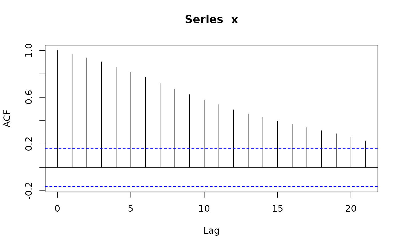
x <- sim_sarima(n=144, model = list(iorder=1, sigma2 = 1)) # (1-B)X_t = e_t (random walk)
acf(x)
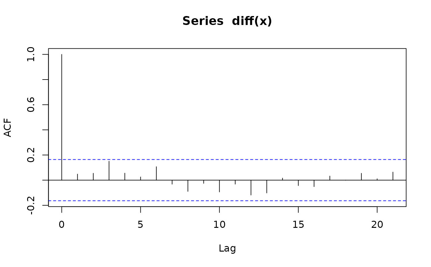
 acf(diff(x))
 x <- sim_sarima(n=144, model = list(iorder=2, sigma2 = 1)) # (1-B)^2 X_t = e_t
x <- sim_sarima(n=144, model = list(siorder=1,
nseasons=12, sigma2 = 1)) # (1-B)^{12} X_t = e_t
x <- sim_sarima(n=144, model = list(iorder=1, siorder=1,
nseasons=12, sigma2 = 1))
x <- sim_sarima(n=144, model = list(ma=0.4, iorder=1, siorder=1,
nseasons=12, sigma2 = 1))
x <- sim_sarima(n=144, model = list(ma=0.4, sma=0.7, iorder=1, siorder=1,
nseasons=12, sigma2 = 1))
x <- sim_sarima(n=144, model = list(ar=c(1.2,-0.8), ma=0.4,
sar=0.3, sma=0.7, iorder=1, siorder=1,
nseasons=12, sigma2 = 1))
x <- sim_sarima(n=144, model = list(iorder=1, siorder=1,
nseasons=12, sigma2 = 1),
x = list(init=AirPassengers[1:13]))
p <- polynom(c(1,-1.2,0.8))
solve(p)
#> [1] 0.75-0.8291562i 0.75+0.8291562i
abs(solve(p))
#> [1] 1.118034 1.118034
sim_sarima(n=144, model = list(ar=c(1.2,-0.8), ma=0.4, sar=0.3, sma=0.7,
iorder=1, siorder=1, nseasons=12))
#> [1] 0.0000000 0.0000000 0.0000000 0.0000000 0.0000000
#> [6] 0.0000000 0.0000000 0.0000000 0.0000000 0.0000000
#> [11] 0.0000000 0.0000000 0.0000000 0.0000000 0.0000000
#> [16] 0.0000000 0.0000000 0.0000000 0.0000000 0.0000000
#> [21] 0.0000000 0.0000000 0.0000000 0.0000000 0.0000000
#> [26] 0.0000000 0.0000000 0.1724162 1.8191105 4.4951421
#> [31] 7.7565445 11.4980009 12.6423926 9.8891186 6.9972791
#> [36] 4.8772707 3.5041348 3.9426081 7.5538477 12.0052028
#> [41] 16.0912819 18.4013656 21.8425941 27.3745515 27.1230466
#> [46] 19.2559338 13.2075814 11.0343077 11.7294921 15.1923258
#> [51] 23.6960551 33.4628693 40.7847508 43.0180781 46.1361142
#> [56] 51.1640328 47.3970227 34.0316649 25.1417253 23.0349050
#> [61] 27.6035443 35.9087677 48.8440147 60.5553281 66.7411521
#> [66] 65.1774147 64.4136176 65.6475543 58.9513993 42.9666951
#> [71] 33.3288394 32.4003219 39.9719180 52.7790921 70.9891916
#> [76] 84.1398829 87.5740936 79.7507837 70.4716697 63.4703631
#> [81] 52.8261267 37.1946893 30.3301536 33.7707998 44.0232098
#> [86] 56.9964641 72.6333310 81.0005855 80.0381422 69.4874834
#> [91] 56.1410554 42.5697739 25.6724533 7.4528564 1.2950855
#> [96] 10.8833122 28.4799076 44.6569911 57.1675387 59.0741944
#> [101] 51.3925223 35.5015748 16.9311209 -1.3164451 -20.8773496
#> [106] -36.9635997 -38.1281286 -21.1657024 2.8171803 21.0717162
#> [111] 31.1198506 27.7276406 16.2040795 -2.5995738 -23.9848763
#> [116] -45.4596366 -66.4651792 -80.3087614 -75.9940561 -51.7663846
#> [121] -23.9730144 -7.8511855 -3.8292833 -15.2040259 -29.5410071
#> [126] -45.7776925 -62.3336774 -81.4535313 -102.9191513 -119.3549942
#> [131] -116.3438834 -89.8340741 -59.3806523 -41.3307688 -36.4498937
#> [136] -51.2301545 -69.7100193 -88.3789172 -103.2578737 -117.5078036
#> [141] -132.6115490 -144.8983306 -140.0161477 -113.7587376
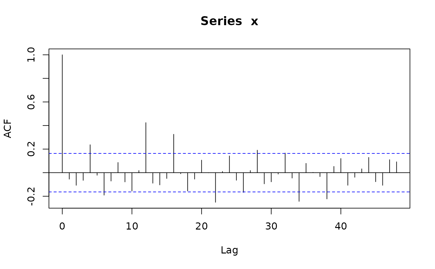
x <- sim_sarima(n=144, model=list(ma=0.4, iorder=1, siorder=1, nseasons=12))
acf(x, lag.max=48)
x <- sim_sarima(n=144, model = list(iorder=2, sigma2 = 1)) # (1-B)^2 X_t = e_t
x <- sim_sarima(n=144, model = list(siorder=1,
nseasons=12, sigma2 = 1)) # (1-B)^{12} X_t = e_t
x <- sim_sarima(n=144, model = list(iorder=1, siorder=1,
nseasons=12, sigma2 = 1))
x <- sim_sarima(n=144, model = list(ma=0.4, iorder=1, siorder=1,
nseasons=12, sigma2 = 1))
x <- sim_sarima(n=144, model = list(ma=0.4, sma=0.7, iorder=1, siorder=1,
nseasons=12, sigma2 = 1))
x <- sim_sarima(n=144, model = list(ar=c(1.2,-0.8), ma=0.4,
sar=0.3, sma=0.7, iorder=1, siorder=1,
nseasons=12, sigma2 = 1))
x <- sim_sarima(n=144, model = list(iorder=1, siorder=1,
nseasons=12, sigma2 = 1),
x = list(init=AirPassengers[1:13]))
p <- polynom(c(1,-1.2,0.8))
solve(p)
#> [1] 0.75-0.8291562i 0.75+0.8291562i
abs(solve(p))
#> [1] 1.118034 1.118034
sim_sarima(n=144, model = list(ar=c(1.2,-0.8), ma=0.4, sar=0.3, sma=0.7,
iorder=1, siorder=1, nseasons=12))
#> [1] 0.0000000 0.0000000 0.0000000 0.0000000 0.0000000
#> [6] 0.0000000 0.0000000 0.0000000 0.0000000 0.0000000
#> [11] 0.0000000 0.0000000 0.0000000 0.0000000 0.0000000
#> [16] 0.0000000 0.0000000 0.0000000 0.0000000 0.0000000
#> [21] 0.0000000 0.0000000 0.0000000 0.0000000 0.0000000
#> [26] 0.0000000 0.0000000 0.1724162 1.8191105 4.4951421
#> [31] 7.7565445 11.4980009 12.6423926 9.8891186 6.9972791
#> [36] 4.8772707 3.5041348 3.9426081 7.5538477 12.0052028
#> [41] 16.0912819 18.4013656 21.8425941 27.3745515 27.1230466
#> [46] 19.2559338 13.2075814 11.0343077 11.7294921 15.1923258
#> [51] 23.6960551 33.4628693 40.7847508 43.0180781 46.1361142
#> [56] 51.1640328 47.3970227 34.0316649 25.1417253 23.0349050
#> [61] 27.6035443 35.9087677 48.8440147 60.5553281 66.7411521
#> [66] 65.1774147 64.4136176 65.6475543 58.9513993 42.9666951
#> [71] 33.3288394 32.4003219 39.9719180 52.7790921 70.9891916
#> [76] 84.1398829 87.5740936 79.7507837 70.4716697 63.4703631
#> [81] 52.8261267 37.1946893 30.3301536 33.7707998 44.0232098
#> [86] 56.9964641 72.6333310 81.0005855 80.0381422 69.4874834
#> [91] 56.1410554 42.5697739 25.6724533 7.4528564 1.2950855
#> [96] 10.8833122 28.4799076 44.6569911 57.1675387 59.0741944
#> [101] 51.3925223 35.5015748 16.9311209 -1.3164451 -20.8773496
#> [106] -36.9635997 -38.1281286 -21.1657024 2.8171803 21.0717162
#> [111] 31.1198506 27.7276406 16.2040795 -2.5995738 -23.9848763
#> [116] -45.4596366 -66.4651792 -80.3087614 -75.9940561 -51.7663846
#> [121] -23.9730144 -7.8511855 -3.8292833 -15.2040259 -29.5410071
#> [126] -45.7776925 -62.3336774 -81.4535313 -102.9191513 -119.3549942
#> [131] -116.3438834 -89.8340741 -59.3806523 -41.3307688 -36.4498937
#> [136] -51.2301545 -69.7100193 -88.3789172 -103.2578737 -117.5078036
#> [141] -132.6115490 -144.8983306 -140.0161477 -113.7587376
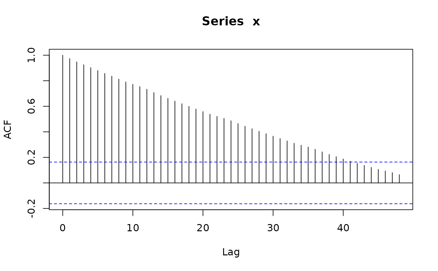
x <- sim_sarima(n=144, model=list(ma=0.4, iorder=1, siorder=1, nseasons=12))
acf(x, lag.max=48)
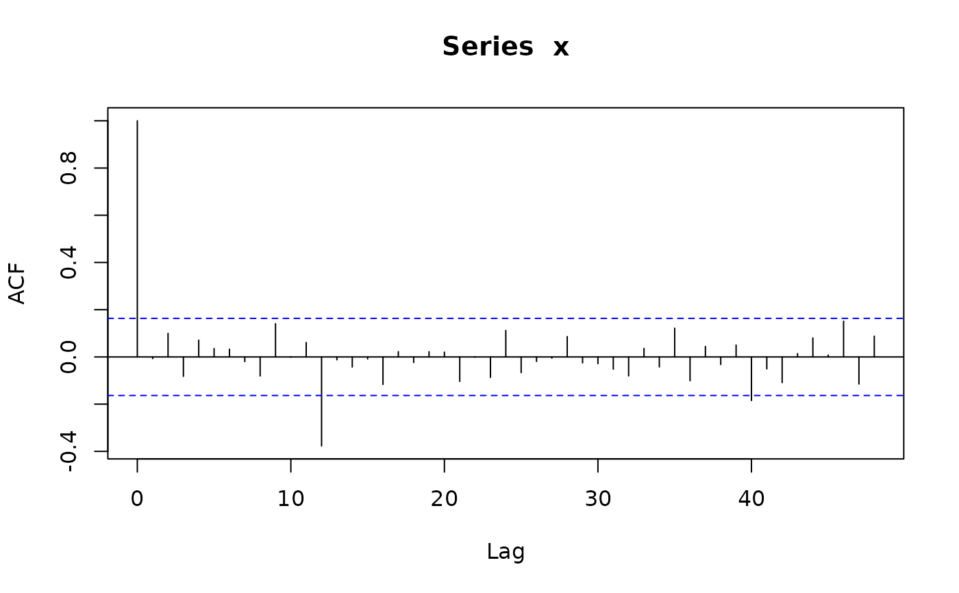
 x <- sim_sarima(n=144, model=list(sma=0.4, iorder=1, siorder=1, nseasons=12))
acf(x, lag.max=48)
x <- sim_sarima(n=144, model=list(sma=0.4, iorder=1, siorder=1, nseasons=12))
acf(x, lag.max=48)
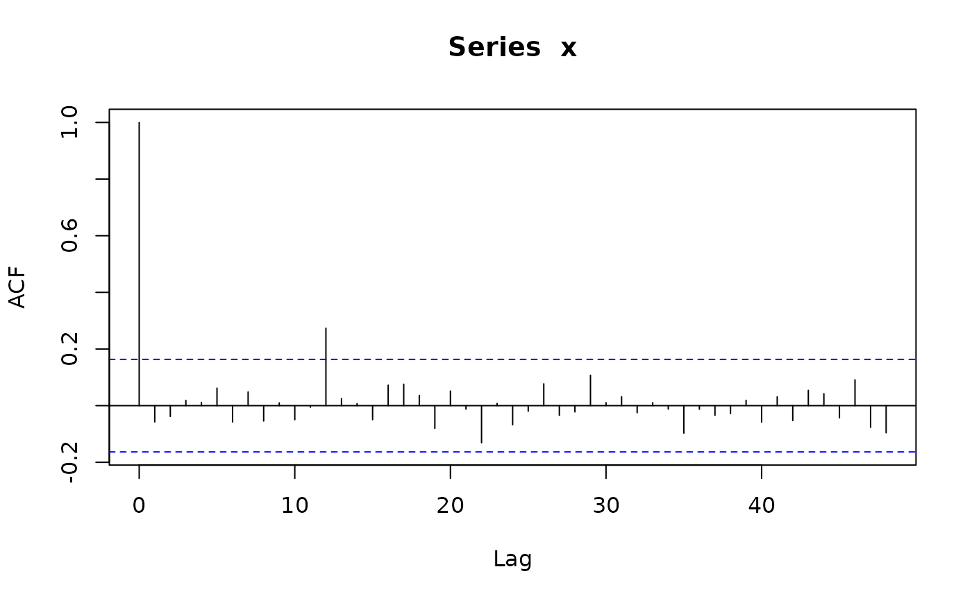
 x <- sim_sarima(n=144, model=list(sma=0.4, iorder=0, siorder=0, nseasons=12))
acf(x, lag.max=48)
x <- sim_sarima(n=144, model=list(sma=0.4, iorder=0, siorder=0, nseasons=12))
acf(x, lag.max=48)
 x <- sim_sarima(n=144, model=list(sar=0.4, iorder=0, siorder=0, nseasons=12))
acf(x, lag.max=48)
x <- sim_sarima(n=144, model=list(sar=0.4, iorder=0, siorder=0, nseasons=12))
acf(x, lag.max=48)
 x <- sim_sarima(n=144, model=list(sar=-0.4, iorder=0, siorder=0, nseasons=12))
acf(x, lag.max=48)
x <- sim_sarima(n=144, model=list(sar=-0.4, iorder=0, siorder=0, nseasons=12))
acf(x, lag.max=48)
 x <- sim_sarima(n=144, model=list(ar=c(1.2, -0.8), ma=0.4, sar=0.3, sma=0.7,
iorder=1, siorder=1, nseasons=12))
## use xintercept to include arbitrary trend/covariates
sim_sarima(n = 144, model = list(sma = 0.4, ma = 0.4, sar = 0.8, ar = 0.5,
nseasons = 12, sigma2 = 1), xintercept = 1:144)
#> [1] -2.1461016 -1.4891387 -0.4078933 2.2886570 0.6755563 -0.3102220
#> [7] -0.8142428 -0.9689355 -3.5960172 -3.1248383 -2.6062497 -2.8400135
#> [13] -2.1256047 11.9094415 19.7567539 28.5178831 30.0438121 33.5759352
#> [19] 35.4122264 36.8401710 36.5895983 38.2088620 39.7584226 43.0043981
#> [25] 45.8327279 58.2397101 65.7340500 74.9334957 76.8157773 82.4298005
#> [31] 87.5226703 91.6669206 94.2428586 97.2973871 99.5370678 105.3780248
#> [37] 109.5190590 120.7336107 128.8949223 137.1487882 138.6252715 145.5954941
#> [43] 152.6091945 158.9040716 165.7149108 171.0091528 173.3630452 181.7217368
#> [49] 187.9540497 197.4574229 204.4537625 212.0634804 214.1714191 220.8593514
#> [55] 226.9397476 234.7625188 242.7476025 250.8789981 253.6823932 264.4878770
#> [61] 271.7631993 278.9931238 286.1764589 293.7123641 298.2367433 308.2717398
#> [67] 314.1801728 322.0563573 330.6252158 339.9172093 343.7181023 355.4614569
#> [73] 362.4713701 371.0649804 379.0994767 386.6083913 393.6681186 403.5215265
#> [79] 408.7359517 416.7860551 425.5312845 434.5839601 438.0941003 448.6127197
#> [85] 458.0702276 469.2617365 478.4345738 486.8826292 493.4465134 501.3432968
#> [91] 506.8039153 516.0017700 525.2290142 534.9759370 538.8131544 550.3558302
#> [97] 559.7974928 568.8627353 577.1182670 586.1986237 593.2753396 601.3631821
#> [103] 610.1223290 622.4949412 632.4467767 641.4825570 644.8896431 656.6533666
#> [109] 667.2467434 673.9915671 682.4763849 689.6972364 697.3010446 708.1278366
#> [115] 717.8402720 730.7457609 739.9243523 748.8903377 752.3582050 762.3901845
#> [121] 773.4121774 780.4905820 790.3725771 798.4905145 809.7143811 821.0743213
#> [127] 829.3444613 839.5700103 847.1976702 855.9355059 862.3534774 872.3205948
#> [133] 881.9431626 887.5647498 898.9524857 908.2990875 920.6832114 932.9809209
#> [139] 941.6063657 950.3792157 959.2521852 969.0425863 975.4049226 984.2753883
x <- sim_sarima(n=144, model=list(ar=c(1.2, -0.8), ma=0.4, sar=0.3, sma=0.7,
iorder=1, siorder=1, nseasons=12))
## use xintercept to include arbitrary trend/covariates
sim_sarima(n = 144, model = list(sma = 0.4, ma = 0.4, sar = 0.8, ar = 0.5,
nseasons = 12, sigma2 = 1), xintercept = 1:144)
#> [1] -2.1461016 -1.4891387 -0.4078933 2.2886570 0.6755563 -0.3102220
#> [7] -0.8142428 -0.9689355 -3.5960172 -3.1248383 -2.6062497 -2.8400135
#> [13] -2.1256047 11.9094415 19.7567539 28.5178831 30.0438121 33.5759352
#> [19] 35.4122264 36.8401710 36.5895983 38.2088620 39.7584226 43.0043981
#> [25] 45.8327279 58.2397101 65.7340500 74.9334957 76.8157773 82.4298005
#> [31] 87.5226703 91.6669206 94.2428586 97.2973871 99.5370678 105.3780248
#> [37] 109.5190590 120.7336107 128.8949223 137.1487882 138.6252715 145.5954941
#> [43] 152.6091945 158.9040716 165.7149108 171.0091528 173.3630452 181.7217368
#> [49] 187.9540497 197.4574229 204.4537625 212.0634804 214.1714191 220.8593514
#> [55] 226.9397476 234.7625188 242.7476025 250.8789981 253.6823932 264.4878770
#> [61] 271.7631993 278.9931238 286.1764589 293.7123641 298.2367433 308.2717398
#> [67] 314.1801728 322.0563573 330.6252158 339.9172093 343.7181023 355.4614569
#> [73] 362.4713701 371.0649804 379.0994767 386.6083913 393.6681186 403.5215265
#> [79] 408.7359517 416.7860551 425.5312845 434.5839601 438.0941003 448.6127197
#> [85] 458.0702276 469.2617365 478.4345738 486.8826292 493.4465134 501.3432968
#> [91] 506.8039153 516.0017700 525.2290142 534.9759370 538.8131544 550.3558302
#> [97] 559.7974928 568.8627353 577.1182670 586.1986237 593.2753396 601.3631821
#> [103] 610.1223290 622.4949412 632.4467767 641.4825570 644.8896431 656.6533666
#> [109] 667.2467434 673.9915671 682.4763849 689.6972364 697.3010446 708.1278366
#> [115] 717.8402720 730.7457609 739.9243523 748.8903377 752.3582050 762.3901845
#> [121] 773.4121774 780.4905820 790.3725771 798.4905145 809.7143811 821.0743213
#> [127] 829.3444613 839.5700103 847.1976702 855.9355059 862.3534774 872.3205948
#> [133] 881.9431626 887.5647498 898.9524857 908.2990875 920.6832114 932.9809209
#> [139] 941.6063657 950.3792157 959.2521852 969.0425863 975.4049226 984.2753883