Plot methods in package sarima
plot-methods.RdPlot methods in package sarima.
Methods
signature(x = "SampleAutocorrelations", y = "matrix")signature(x = "SampleAutocorrelations", y = "missing")-
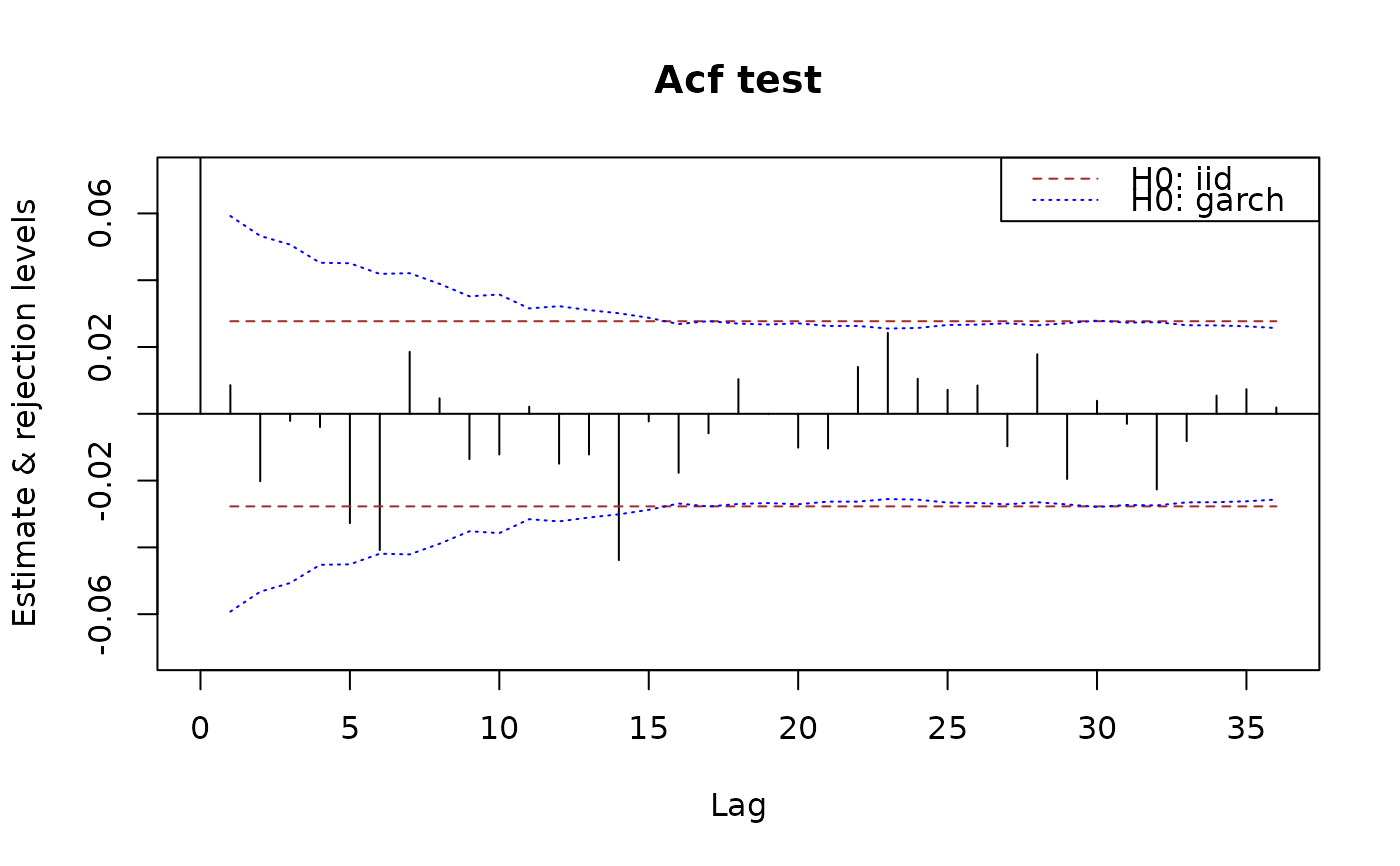
plots the sample autocorrelations with (individual) rejection limits computed under the null hypothesis of i.i.d. (strong white noise) If argument
datais provided, it should be the time series from which the autocorrelations were computed. In this case rejection limits for null hypothesis that the time series is (garch) weak white noise are provided, as well.Additional arguments can be supplied, see
whiteNoiseTestthe examples, and the vignettes. signature(x = "SamplePartialAutocorrelations", y = "missing")-
plots the sample partial autocorrelations with rejection limits for the hypotheses and controlling arguments as for
"SampleAutocorrelations".
See also
whiteNoiseTest for the computations for the rejection
levels;
Examples
set.seed(1234)
n <- 5000
x <- sarima:::rgarch1p1(n, alpha = 0.3, beta = 0.55, omega = 1, n.skip = 100)
x.acf <- autocorrelations(x)
x.acf
#> An object of class "SampleAutocorrelations"
#> Lag_0 Lag_1 Lag_2 Lag_3 Lag_4
#> 1.000000e+00 8.582362e-03 -2.018313e-02 -2.132628e-03 -3.961602e-03
#> Lag_5 Lag_6 Lag_7 Lag_8 Lag_9
#> -3.274167e-02 -4.079434e-02 1.854328e-02 4.641011e-03 -1.357080e-02
#> Lag_10 Lag_11 Lag_12 Lag_13 Lag_14
#> -1.219076e-02 2.136221e-03 -1.492981e-02 -1.219485e-02 -4.381421e-02
#> Lag_15 Lag_16 Lag_17 Lag_18 Lag_19
#> -2.281830e-03 -1.766486e-02 -5.846757e-03 1.037726e-02 -9.286768e-05
#> Lag_20 Lag_21 Lag_22 Lag_23 Lag_24
#> -1.013180e-02 -1.038853e-02 1.402807e-02 2.423647e-02 1.047997e-02
#> Lag_25 Lag_26 Lag_27 Lag_28 Lag_29
#> 7.201460e-03 8.488189e-03 -9.712715e-03 1.784192e-02 -1.952790e-02
#> Lag_30 Lag_31 Lag_32 Lag_33 Lag_34
#> 3.907283e-03 -3.013057e-03 -2.266969e-02 -8.177097e-03 5.453303e-03
#> Lag_35 Lag_36
#> 7.377188e-03 1.883301e-03
#> Slot n:
#> [1] 5000
#> Slot varnames: <not set>
#> Slot objectname: x
x.pacf <- partialAutocorrelations(x)
x.pacf
#> An object of class "SamplePartialAutocorrelations"
#> Lag_0 Lag_1 Lag_2 Lag_3 Lag_4
#> 1.0000000000 0.0085823617 -0.0202582774 -0.0017828992 -0.0043383782
#> Lag_5 Lag_6 Lag_7 Lag_8 Lag_9
#> -0.0327650792 -0.0404641407 0.0178960591 0.0025478441 -0.0134144032
#> Lag_10 Lag_11 Lag_12 Lag_13 Lag_14
#> -0.0132073022 -0.0006562451 -0.0160165907 -0.0104612044 -0.0454777643
#> Lag_15 Lag_16 Lag_17 Lag_18 Lag_19
#> -0.0042317566 -0.0202992932 -0.0065655314 0.0070365865 -0.0043112264
#> Lag_20 Lag_21 Lag_22 Lag_23 Lag_24
#> -0.0136537970 -0.0107137774 0.0114656459 0.0228629885 0.0098952431
#> Lag_25 Lag_26 Lag_27 Lag_28 Lag_29
#> 0.0058602874 0.0053481194 -0.0098438262 0.0191055268 -0.0192762938
#> Lag_30 Lag_31 Lag_32 Lag_33 Lag_34
#> 0.0032466133 -0.0038284295 -0.0219232817 -0.0081774145 0.0051229039
#> Lag_35 Lag_36
#> 0.0052288057 0.0036772670
#> Slot n:
#> [1] 5000
#> Slot varnames: <not set>
#> Slot objectname: x
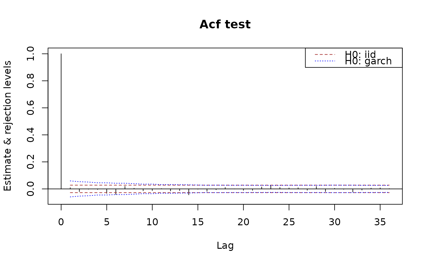
plot(x.acf)
 ## add limits for a weak white noise test:
plot(x.acf, data = x)
## add limits for a weak white noise test:
plot(x.acf, data = x)
 ## similarly for pacf
plot(x.pacf)
## similarly for pacf
plot(x.pacf)
 plot(x.pacf, data = x)
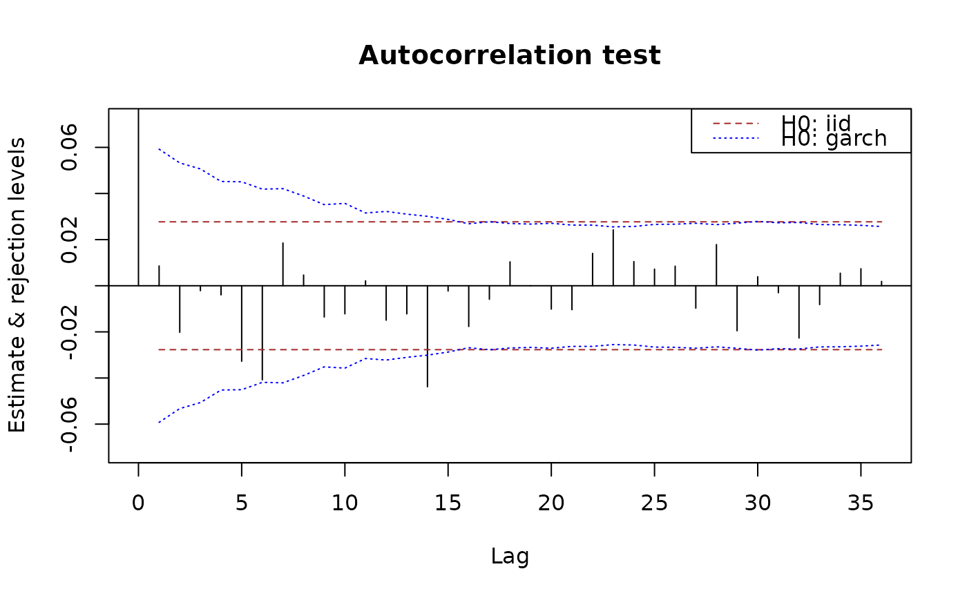
 plot(x.acf, data = x, main = "Autocorrelation test")
 plot(x.pacf, data = x, main = "Partial autocorrelation test")
 plot(x.acf, ylim = c(NA,1))
 plot(x.acf, ylim.fac = 1.5)
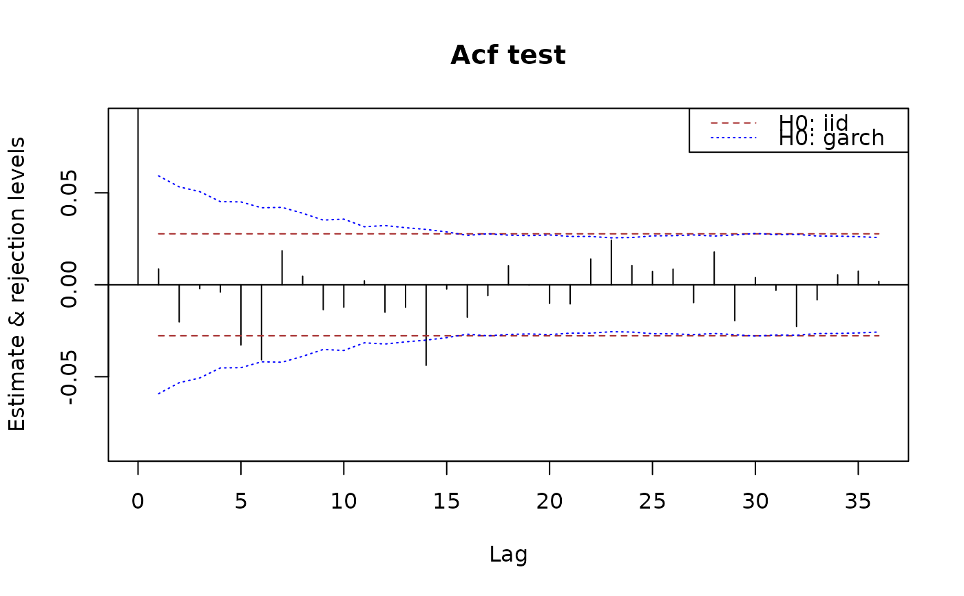
 plot(x.acf, data = x, ylim.fac = 1.5)
 plot(x.acf, data = x, ylim = c(NA, 1))