Simulate periodically correlated ARMA series

Simulate a realization of a periodically correlated arma model or a continuation of an existing series. Initial values may be given too.

Usage

sim_pc(model, n = NA, randgen = rnorm, seasonof1st = 1, nepochs = NA,
              n.start = NA, x, eps, nmean = NULL, nintercept = NULL, ...)

Arguments

model: a list with elements phi, theta, p, q, period, mean, intercept, specifying the model.
n: length of the series.
randgen: random number generator as required by sim_pwn.

seasonof1st: season of the first value.
nepochs: number of epochs; if nepochs is given, then n is computed as $nepochs * period$.
n.start: burn-in number; generate $\code{n.start + n}$ observations and discard the first n.start of them, see Details.
x: initial or before values, see Details.
eps: innovations, see Details.
nmean: a vector of length n of means, see Details.
nintercept: a vector of length n of intercepts, see Details.
...: any additional arguments to be passed on to sim_pwn.

Details

Argument x can be used to specify two types of initialisation values - `before' and `init'. They are used similarly in computations but `before' values are not included in the result, while `init' values are (unless dropped due to n.start). `Before' values provide a convenient way to simulate continuation trajectories for a time series, for example for simulation based prediction intervals.

If x is "numeric", it represents `before' values. Alternatively, x can be a list with components "before" and "init".

Innovations are usually generated with the random number generator specified by randgen (with default rnorm) and the ... parameters by a call to the function sim_pwn, see the documentation for sim_pwn for various ways to control the distribution of the generated sequence.

The innovations can also be generated in advance and supplied using argument eps. If eps is numeric, it is taken to represent the innovations. Alternatively, eps can be a list with the innovations in component "main". This list may also contain components "before" and/or "init" specifying `before' or `initial' values, with interpretation as for x.

nintercept can be used to specify trend representing the effect of time and/or covariates. As for eps, if it is numeric it is taken to represent the main values. It can also be a list with components before, init, and main.

To avoid ambiguity, let's reiterate that before values are past values of the corresponding quantity (before the start of the simulated series), while init values are "initial" values. In particular, if initial values are specified for x, these will form the start of the generated series (unless n.start leads to them being discarded).

If before values are specified for the series and the innovations, then they play a role analogous to that of initial values, so it does not make much sense to supply also initial values.

The function effectively does the following. innov is generated if not supplied, a vector of innovations is created eps <- c(innovbefore,innovinit,innov), a vector x is created of the same length as eps, and initialised with xbefore and xinit. If there are no initial or before values, these are assumed to be 0. The remaining values of x are filled using the pc-arma equations. Finally, the xbefore values are discarded as well as the first n.start values.

n.start should usually be a multiple of the period since otherwise the first observation in the returned vector will not correspond to seasonof1st.

sim_pc deals mainly with the interpretation of the parameters. The actual computations are done by pc.filter. Moreover, sim_pc does not look at the model. It knows only about model$period and uses it to compute n if n is not specified. (It probably should not care even about this.)

Value

numeric, the simulated time series

Author

Georgi N. Boshnakov

To do

option to return the innovation sequence; option to include the before values.

option to return the season of the first value in the returned series (it may be different from seasonof1st due to n.start).

Examples

m1 <- rbind( c(1, 0.81, 0), c(1, 0.4972376, 0.4972376) )
testphi <- slMatrix( init = m1 )

m2 <- rbind( c(1, 0, 0), c(1, 0, 0) )
testtheta <- slMatrix( init = m2 )

## phi and theta are slMatrix here.
mo1 <- list(phi = testphi, theta = testtheta, p = 2, q = 2, period = 2)
set.seed(1234)
a1 <- sim_pc(mo1, 100)

## phi and theta are ordinary matrices here.
mo2 <- list(phi = m1[ , 2:ncol(m1)], theta = m2[ , 2:ncol(m2)], p = 2, q = 2, period = 2)
set.seed(1234)
a2 <- sim_pc(mo2, 100)
identical(a1, a2)
#> [1] TRUE

## Lina's PAR model
parcoef    <- rbind(c(0.5, -0.06), c(0.6, -0.08),
                    c(0.7, -0.1),  c(0.2, 0.15) )
picoef1    <- c(0.8, 1.25, 2, 0.5)
parcoef2   <- pi1ar2par(picoef1, parcoef)

picoef2    <- c(4, 0.25, 5, 0.2)
coefper2I2 <- pi1ar2par(picoef2, parcoef2)

#### specify the model using multi-companion approach
mc2I2       <- mcompanion::mc_from_filter(coefper2I2)
co2I2       <- eigen(mc2I2)$vectors
co2I2
#>           [,1]       [,2]       [,3]          [,4]
#> [1,] 0.1524986 -0.1524986 0.01157344 -0.0005488947
#> [2,] 0.7624929 -0.7624928 0.26297482  0.0405688010
#> [3,] 0.1524986 -0.1524986 0.09131096  0.0323513211
#> [4,] 0.6099942 -0.6099943 0.96040232  0.9986527240
m2I2 <-  mcompanion::sim_pcfilter(period = 4, n.root = 4,
                 eigabs = c(1, 0.036568887, 0.001968887),
                 eigsign = c(1, 1, -1),
                 len.block = c(2, 1, 1),
                 type.eigval  =  c("r", "r", "r"),
                 co = cbind(co2I2[ ,1], rep(NA, 4), co2I2[,3:4]))
m2I2$pcfilter
#>            [,1]         [,2]        [,3]        [,4]
#> [1,] 26.6776382 -11.62777150 38.51128378 -0.76251650
#> [2,]  0.3204255  -0.08629939 -0.05644545  0.08682460
#> [3,]  7.4995587  -1.47779772  3.48496388 -0.01466647
#> [4,]  0.4794181  -1.52298674  0.05001173 -0.07415064
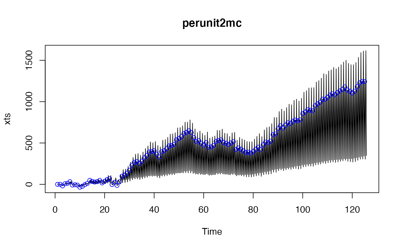
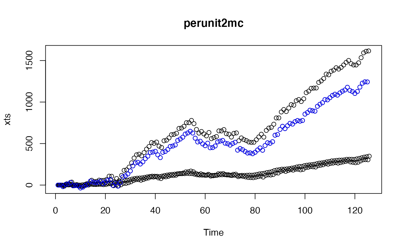
perunit2mc  <- sim_pc(list(phi = m2I2$pcfilter, p = 4, q = 0, period = 4), 500)
plot(perunit2mc)

plot(perunit2mc, type = "p")


# todo: give example with sigmat^2 !!!