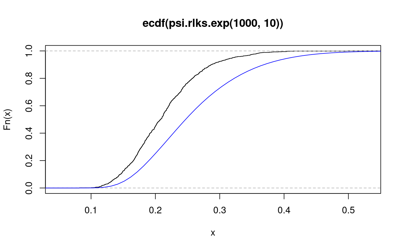
Approximate distribution of the Lilliefors's statistic for exponential hypotheses

Distribution function, quantile function and random generation for the distribution of the Lilliefors's statistic for exponential hypotheses.

psi.plks.exp(q, df, Nsim = 1000, lower.tail = TRUE)
psi.qlks.exp(p, df, Nsim = 1000)
psi.rlks.exp(n, df)

Arguments

p	vector of probabilities.
q	vector of quantiles.
df	degrees of freedom of the statistic.
n	number of observations.
Nsim	number of simulations.
lower.tail	if TRUE (default) lower tail, otherwise upper tail.

Details

The prefixes 'p', 'q' and 'r' follow the conventions of distribution functions in base R. The prefix 'psi.' is a reminder that they are in package "psistat".

The distribution function and the quantiles are obtained from a sample of size Nsim, ideally large. So, they should not be expected to give identical results in repeated calls with the same parameters.

Instances of the statistic are obtained by generating random samples of length df from the exponential distribution, transforming each by the formula \(z=x/{\bar x}\), and calculating the Kolmogorov statistic for the transformed sample, \(z\), with \(F_0\) set to the exponential distribution with rate 1.

todo: pdf

Value

for psi.plks.exp, a numeric vector of the same length as the vector q.

for psi.qlks.exp, a numeric vector of the same length as the vector p.

for psi.rlks.exp, a numeric vector of length n representing a sample from the distribution of the Lilliefors KS statistic for the exponential distribution.

See also

lillie.test in package nortest for the Lilliefors test for normality.

Examples

psi.plks.exp(c(0.1,0.2,0.3,0.4), 10, Nsim=1000)
#>   0.1   0.2   0.3   0.4 
#> 0.002 0.428 0.900 0.996 
psi.qlks.exp(c(0.25,0.5,0.75), 10, Nsim=10000)
#>      0.25       0.5      0.75 
#> 0.1736681 0.2081081 0.2506081 

xi <- seq(0,1,length=100)
yi <- psi.qlks.exp(xi,10,Nsim=10000)
plot(xi,yi)


# aproximate cdf of Lilliefors stat.
plot(ecdf(psi.rlks.exp(1000,10)))

# overlay the cdf of Kolmogorov for comparison.
lines(seq(0,1,length=100), psi.pks(seq(0,1,length=100),10),col="blue")